Revolutionary Progress of Zero-Knowledge Proof Technology In-depth Exploration of the Nova Algorithm

Zero-Knowledge Proof Technology and Nova Algorithm Revolutionary Progress and In-depth Exploration.

A while ago I was translating a book on zero-knowledge proof technology. The basic content was translated by the end of last month. The translation took much longer than I expected. I am currently discussing some typos with the author and preparing for the final draft.

Anyway, I finally have some time to look at something new. Let’s start with the Nova algorithm~

Resources related to the Nova algorithm

Three resources can help understand the Nova algorithm:

• Restaking King Is EigenLayer’s business model a great idea or a waste?
• IDO&IEO Inventory of 8 Hot Projects to Be Launched Soon (September First Wave)
• Financial History, Legal System, and Technological Cycle The Trillion Dollar Narrative of RWA Cannot Withstand Scrutiny

1. Nova paper: https://eprint.iacr.org/2021/370.pdf

1. Potential attacks and corresponding fixes for Nova: https://eprint.iacr.org/2023/969.pdf

2. Summary of understanding potential attacks on Nova: https://www.zksecurity.xyz/blog/posts/nova-attack/

This article is an understanding and summary of the above resources. Some of the figures in this article come from the above resources and will not be individually marked in this article.

Starting from IVC

The Nova algorithm is a new zero-knowledge proof algorithm for IVC (Incrementally Verifiable Computation). IVC refers to the iterative computation of the same function with the previous output as the next input. The iterative computation process of the F function is as shown in the following figure:

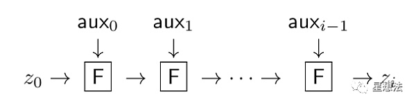
z0 is the initial input, and the result generated by the F function is used as the input for the next F function.

Relaxed R1CS and Relaxed Commitment R1CS

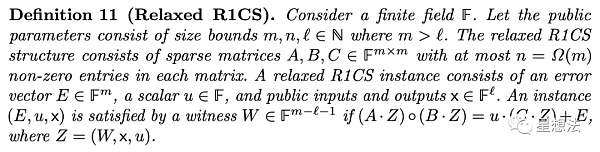
It is well known that R1CS is a circuit constraint representation form in zero-knowledge proof technology. Relaxed R1CS can be seen as an extended form of R1CS. Based on R1CS, a scalar u and an error vector E are added. Instances of relaxed R1CS are represented as (E, u, x).

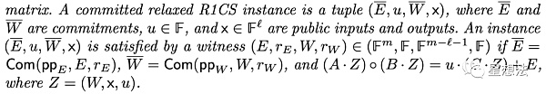
Relaxed Commitment R1CS is based on relaxed R1CS and commits to the E and W vectors. Instances of relaxed commitment R1CS are represented as (\bar{E}, u, \bar{W}, x), where x and u are public variables.

Folding from R1CS to relaxed R1CS is for the purpose of folding schemes. It should be noted that from the perspective of relaxed R1CS, R1CS is a special case of it. In other words, R1CS is also a “special” relaxed R1CS.

Folding Scheme

Intuitively, a folding scheme for a relation R is to “fold” two instances that satisfy relation R into a new composite instance that satisfies relation R. Both relaxed R1CS and relaxed commitment R1CS can perform similar folding. The folding process for relaxed commitment R1CS is as follows:

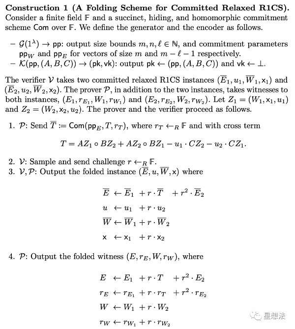
The entire folding scheme consists of 4 steps. In the first step, the prover P sends a commitment \bar{T} for the cross-term T to the verifier. In the second step, the verifier sends a random challenge r to the prover. The third step is performed by both the prover and the verifier, which is the folding of commitments. In the fourth step, performed solely by the prover, the E and W vectors of the two instances are folded.

Augmented Function F’ (Argumented Function)

Folding scheme, folding the relaxed R1CS instance. What is the calculation proved by these relaxed R1CS instances? Obviously, these calculations include the folded calculation. These calculations are not only the F function in IVC calculation, but also called the augmented function F’. The calculation of augmented function F’ mainly consists of two parts:

1/ F function in IVC

2/ Folding calculation of R1CS instance

What it looks like ideally

With the above understanding, we can imagine the folding process:

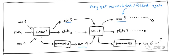
Where circuit is the circuit corresponding to the augmented function F’. acc{1,2,3,4,5,6} is the relaxed commitment R1CS instance. The circuit has two calculations: 1/ Folding of the relaxed commitment R1CS instance, such as acc1+acc2->acc3. 2/ Calculation of the F function, transforming state1 into state2, and then from state2 into state3, and so on.

It should be noted that the circuit corresponding to the augmented function F’ itself is also an R1CS instance, which can be represented as a relaxed R1CS instance. That is, acc4 and acc6 in the figure. “Summarize” is to transform the relaxed R1CS instance into the relaxed commitment R1CS instance.

By carefully observing the input of the second circuit, acc3 is the folded relaxed commitment R1CS instance, and acc4 is the relaxed commitment R1CS instance that proves acc3 is the correct folding result. These two instances will enter the next fold, generating acc5. You can imagine that if acc3 and acc4 are satisfiable relaxed commitment R1CS instances, it means that acc3 is folded from two satisfiable relaxed commitment R1CS instances, that is, acc1 and acc2 are satisfiable relaxed commitment R1CS instances. The reliability can also be deduced step by step, thereby proving that each F function calculation in the circuit is correct. In summary, the satisfiability of two relaxed commitment R1CS instances corresponding to a certain circuit can prove that all previous IVC calculations are correct.

What it looks like in reality

Friends who are familiar with zero-knowledge proofs know that elliptic curves are often used in polynomial commitment schemes. The commitment of the polynomial corresponding to the scalar field in the scalar field is represented by the base field of the elliptic curve. R1CS circuits are usually represented in the scalar field. Looking closely, the “summarize” before and after in the above figure involves field conversion. That is, in order to fold the relaxed commitment R1CS instance corresponding to the circuit, it must be “folded” in another circuit. At this time, elliptic curve cycles need to be introduced, with two or more elliptic curves, one of which has the same scalar field as the base field of the other curve. Interestingly, the scalar field of this curve is the same as the base field of the previous curve. By using such elliptic curve cycles, the “ideal form” can be realized.

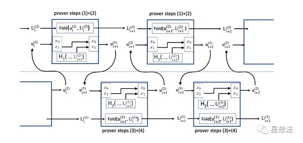
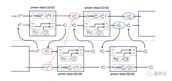
The entire folding process is divided into two circuits for folding. The upper part can be called the folding of Circuit 1, and the lower part can be called the folding of Circuit 2. The formal representation of the relationship between the two circuits is on page 8 of the paper “Nova Potential Attacks and Corresponding Corrections”. U represents the folded instance, u represents the relaxed instance corresponding to an R1CS instance. Note that Circuit 1 folds the relaxed commitment R1CS instance corresponding to Circuit 2, while Circuit 2 folds the relaxed commitment R1CS instance corresponding to Circuit 1. The main purpose of Circuit 2 is to fold the relaxed commitment R1CS instance corresponding to Circuit 1, and the function calculation in its circuit is meaningless. On the contrary, the F function is implemented in Circuit 1. Combining with the “ideal appearance,” it can be roughly guessed that the satisfiability of U{i+2}^2, u{i+2}^1, u{i+2}^2, U{i+2}^1 is an important part of the proof.

Because the “circuit” is divided into two parts and each circuit is folded in the other circuit, there are binding problems between several instances: the binding between u and U instances and the binding of u instances passed between the two circuits. To solve these binding problems, x_0/x_1 public variables are introduced in the circuit, where x_1 specifies the output U instance bound to the u instance and the current output of the F function (not shown in the figure for simplicity of the circuit structure). You see, if the H_1 result of the U instance is introduced in the circuit, if the u instance is satisfiable, x_0/x_1 is both true and reliable, that is, it is “bound” to U. x_0 establishes the binding relationship between the input u and U, and x_1 establishes the binding relationship between the output u and U.

For example, when u{i+1}^1 is used as the input of the lower part of the circuit, after Circuit 2, its output u{i+1}^2.x0 = u{i+1}^1.x1. In this way, when it is input into the upper part of the circuit, if u{i+1}^2 is satisfiable, its x_0 should be equal to the H1 result of U_{i+1}^2. This will be checked in Circuit 1. This ensures the correct instances are passed between the two circuits.

Proof of IVC

In order to prove that IVC correctly calculates in a certain iteration, it is logically necessary to prove the following information:

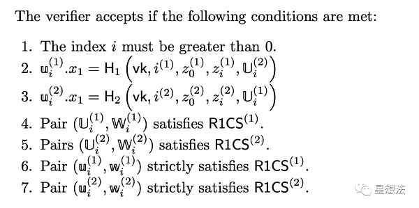
In addition to proving the satisfiability of the four instances, it is also necessary to prove the binding relationship of the two x1s, as shown in the diagram below:

To determine if this information is correct, additional proof circuits are required. In other words, the proof of IVC calculation is the proof of the circuit. As can be imagined, if it is a calculation of many iterations, instead of expanding these iterations one by one in the circuit, it is now only necessary to verify the satisfiability and binding relationships of the four circuit instances. The performance improvement is significant.

Attacks and Algorithm Corrections

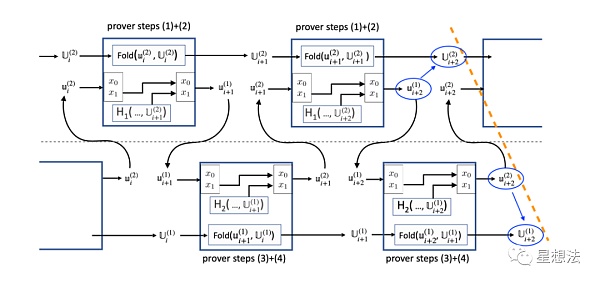
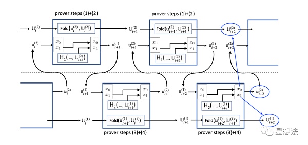
Looking at the above diagram, there is an intuition that the instances of the upper and lower circuits are “separated” and have no binding. In fact, attacks are constructed in this way.

By forging U_i^1 and U{i+1}^2, although they are forged, they are satisfiable instances. By forging u{i+1}^1, the corresponding x_0 and x_1 are modified to match the forged U instance. Obviously, the u{i+1}^1 instance is unsatisfiable. Although it is unsatisfiable, the circuit of Circuit 2 can still be satisfied, only the output instance U{i+1}^1 is unsatisfiable. If u{i+1}^2 is successfully constructed, Circuit 1 can construct a satisfiable u{i+2}^1 and U_{i+2}^2, and satisfy the binding relationship of x1. This way, half of the final forged proof is constructed. By symmetry, the output instance of the other half can be constructed. By “concatenating” the results of the two constructions, the proof of IVC calculation can be forged.

The revised check logic is as follows:

Chapter 6 of the paper “Nova Potential Attacks and Corresponding Corrections” provides a detailed security analysis. Interested friends can refer to the original paper for details.

The basic idea of Nova is to fold circuit instances through folding schemes. The logic is quite complicated and requires careful consideration of the circuit folding process and the implementation of binding relationships in the circuit.

One word to describe it: amazing~

We will continue to update Blocking; if you have any questions or suggestions, please contact us!