Analysis | Is the Black-Scholes model for pricing traditional financial derivatives also applicable to Bitcoin?

The financial world is turbulent, chaotic, and disorderly. So many economists believe that market changes are “random walks” and prices are unpredictable, but this is not necessarily a bad thing.

Here we introduce the concept of Gaussian random walk, which is the underlying assumption used by Black-Scholes' option pricing model. This option pricing model treats the time interval of asset price changes as independent variables, and assumes that price or asset returns follow a normal distribution over time. In other words, transactions are evenly distributed over time, daily, weekly, or The volume of transactions per month is large, so according to the Central Limit Theorem, these prices will conform to a normal or Gaussian distribution. When the return distribution of an asset is normally distributed, the probability of occurrence of different returns is known. Understanding these probabilities can provide investors with an idea to better quantify the risks that can arise when holding these assets.

On this basis, we can't help but wonder if this model can be applied to the new asset of Bitcoin. The rise and fall of Bitcoin is a well-known fact, and there is no debate here. The purpose of this paper is to explore how to build a risk framework and examine the application of implied assumptions in the pricing of traditional financial derivatives in Bitcoin.

At the beginning of this paper, we will introduce the derivatives market, outline the Black-Scholes model, discuss the importance and scope of the model, and analyze its limitations according to the impractical conditions of the model's assumptions, and discuss its feasibility in the bitcoin market. Sex. Based on historical data such as the daily return on Bitcoin during the period from January 2016 to August 2019, we compared the results of the Black-Scholes model applied to Bitcoin and the S&P 500, respectively. Finally, the conclusion that “the Black-Scholes model may not be applicable to the cryptocurrency market” is drawn, and from this conclusion, some inspirations for the fast-growing token derivatives market are obtained.

• Binding social media to send Bitcoin with one click, Bottle Pay received $2 million investment
• Babbitt Column | From Highlights to Fall: P2P Brings Revelation to Defi
• Twitter Featured | Blizzard, Bakkt only 71 BTC on the first day of trading? COO: retail investors will arrive soon

Derivatives and hedging risks

 

Suppose you are a corn grower. You want to harvest 5,000 bushels (about 127 tons) of corn and sell them as much as possible. However, prices are affected by market supply and demand, corn selling offers are lower than production costs, and the use of financial derivatives can minimize the losses caused by these conditions.

Assuming the current market price of corn is around $3.50 per bushel, and you want to "lock" the lower price limit of $3, then you can buy a put option at a price of $3 to avoid the possibility of falling below $3. Since the value of the put option increases as the price of the underlying item decreases, the price at which the option is purchased is the cost of the hedge. If the cost of a put option with a strike price of $3 is 10 cents (5,000 bushels * $0.10 = $500) and the production cost of corn is $1 per bushel, then the minimum profit is $9,500 [(3-2) USD* 5000 bushels – $500 = $9,500)].

The above example explains the role of financial derivatives. Of course, this derivative portfolio can become more complex when considering a full set of futures, options, swaps, and so on. The basis of all these portfolios is that markets and prices reflect risks and uncertainties, and derivatives will minimize this uncertainty.

With this basic understanding, we have a special consideration for the price of any derivative product. The premise of the function of the derivative is that it can represent the actual hedging of the uncertainty of the target. How to apply the option for effective investment is a question worth considering.

The actual risk of the option is actually reflected in the actual price of the subject matter. In the example above, if the price of the put option is $2 instead of 10 cents, the price of the corn is $3.5. Then through the Black-Scholes model, the volatility of the corn price at this time can be calculated to be higher than 200% (see note). This figure is unusual for the agricultural market. Based on this, your expectations for the future price of corn. It will also change. Second, even if your expectations remain the same, buying a put option for $2 will greatly reduce profit margins. If the price of corn falls below $3, you will lose money because of the option fee. Third, if your expectations change and the implied volatility of corn prices is credible, the risk of loss can be significant if corn is produced at a cost of $1 per bushel. Therefore, the effectiveness of option pricing is critical, reflecting the market's expectations for the future.

Black-Scholes model

 

The pricing process for an option contract is actually quite mechanical. As we all know, the Black-Scholes model plays a very important role in option pricing and hedging, and investors and exchanges also use this model to determine the Greek value (the greeks) or calculate δ, Vega, θ in options and other portfolios. , γ and other partial derivatives. These partial derivatives are very helpful for the risk management of exchanges/brokers. They are the coefficients that measure the price sensitivity of derivatives. For example, when large-scale cryptographic derivatives exchange Deribit liquidates high-risk positions, their risk engine is actually creating a “delta neutral” hedge position, letting delta positive and negative, so that the combined value is not Affected by changes in the price of the underlying asset.

Since the Black-Scholes model was first published in the Journal of Po Litical Economy in 1973, the Chicago Board Options Exchange (CBOE) traders immediately realized its importance and soon the model program It was applied to the newly opened CBOE, and in 1986 it launched the first "automatic quote" system using the Black-Scholes model (the system instantly updates the trader's option price for the trader). It can be said that the model has made a milestone contribution to the development of modern finance and the enhancement of the influence of financial derivatives on the market.

The Black-Scholes model also has an impact on the encryption market. Recently, the Bitcoin derivatives exchanges LedgerX and Seed CX announced the launch of a physical settlement of Bitcoin derivatives, and any US resident can participate in the trading of real Bitcoin derivatives, which has generated a lot of interest.

The news of the listing of these new derivatives exchanges has led us to think: Can the Black-Scholes model work in the risk management of Bitcoin? If so, how big is this effect?

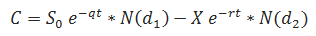
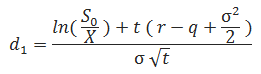
The Black-Scholes model implies the assumption of return on assets, that is, the rate of return is normally distributed, it provides a framework to predict the probability of different returns, investors can do this in the hedging strategy Probability as a reference. Black and Scholes pointed out in their original paper "Pricing of Options and Corporate Liabilities" that the assumption is that "the price of a stock moves randomly over a continuous period of time, and its variance is proportional to the square of the stock price. Therefore, in any finite interval The stock price inside is logarithmic, and the rate of change in stock returns is constant. This assumption can be illustrated by the Black-Scholes formula:

among them:

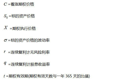
Is the cumulative probability distribution function of a normal distribution variable, representing the part of "value". In the original concept of the model, the "value" part is expressed as the stock price multiplied by function. Later, Robert Merton extended the connotation of the original model and applied it to many other forms of financial transactions.

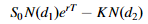
In general, the Black-Scholes formula represents the return on investment Subtract the cost of buying an option. Used to explain the risk-free rate, which is continuously compounded from the time of purchase to the expiration of the option. Essentially, Represents "time value of money", which is the option execution price The present value, in the ideal case, the value of the option should be higher than the current risk-free rate of national debt (T-bill) or government bonds, because if investors can obtain higher returns by purchasing government bonds, then there is no meaning to buy options. It is.

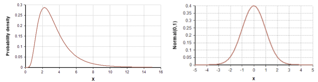
Figure 1: Lognormal distribution (left) and normal distribution (right)

Another point is that the distribution of option prices in the Black-Scholes model is a lognormal distribution. Since the lower bound of the lognormal distribution is zero and the asset price cannot be negative, it is assumed that the price is subject to a lognormal distribution.

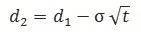
When the option expires It is normally distributed, which means that the distribution of prices is skewed, so the average, median, and mode are not equal.

Represents the daily volatility of asset prices. income Divided by the standard deviation of daily volatility Is a normal distribution. Volatility of assets in the case of a normal distribution of returns Using functions The weighting will determine the distribution curve. Since the volatility is pressed Weighted, so The higher the value, the more "flat" the curve.

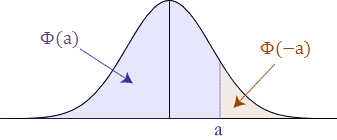
Figure 2: Option execution price probability distribution

When function for At the time, the function represents the probability that the price of the option at the expiration date is higher than the strike price. We can describe this problem through Figure 2. In the case of a call option, if "a" is used to indicate the exercise price, Indicates the expected value of the option when the underlying price increases. When the underlying asset price is less than a, no action is taken, Treated as 0, the value of the call option is 0. When "a" indicates the execution price of the put option, the value of the put option is 0 when the underlying price is greater than a.

on the other hand, Indicates the likelihood that an option will be executed under a risk neutrality measure. Here we can use Figure 2 again to illustrate: assuming that a represents the exercise price, in the call option Indicates the probability that the underlying price is higher than the strike price a; in put options, Indicates the probability that the underlying price is lower than the strike price a.

In the case of continuous compound interest, the Black-Scholes model defines the target asset return rate to be normally distributed by defining the geometrical Brownian motion of the underlying asset price. Determine the probability that an asset price is above or below a given strike price by simulating the probability of an asset's growth rate, ie, calculating the standard deviation between the growth rate of the stock price and the strike price and the expected growth rate. Thereby determining the growth rate. In general, only when the underlying price is greater than the strike price (for call options, the probability is In order to exercise power, in the risk-neutral world, the expected return of the option is:

The higher the volatility, the larger the area of ​​the normal distribution curve and the higher the option price. Therefore, the option price can be considered as a probability distribution.

If the volatility is very stable, and a stock is 100% higher than the exercise price of the call option or 100% lower than the exercise price of the put option when the option expires, then the option has no value. In fact, from the perspective of hedging, it makes no sense to choose an option at this time, because there is no risk to hedge. Or if the stock is 50% more likely to be higher than the call option price or 50% less likely to be lower than the strike price of the put option, then the option is valuable because it can Attract investors to buy options to hedge against the risk of holding underlying stocks.

Defects of the Black-Scholes model

 

The Black-Scholes model is by no means perfect. To some extent, the Black-Scholes model's assumptions about the market do not match the actual situation. Through this model, the trader can obtain the corresponding option price by inputting the parameters such as the strike price, the remaining time due, the underlying asset price, the underlying asset volatility and the risk-free interest rate.

Among the above parameters, the values ​​of four parameters can be accurately obtained from the market, and only the target asset price volatility needs to be estimated. The model assumes that volatility is not only constant, but can be known in advance. This assumption is problematic because the volatility itself may be unstable. CBOE created the Panic Index (VIX), which refers to the implied volatility of the S&P 500 index over the next 30 days. In 2018, the panic index (VIX) fell to a minimum of 8.5% and a maximum of over 46%. Therefore, the volatility throughout the year is not always consistent.

The accuracy of the Black-Scholes model is also affected by market changes. In 1987, the financial market collapsed and the derivatives market was affected at the same time. Prior to 1987, there was little relationship between implied volatility and strike price, and the volatility of the out-of-the-money put and the in-the-money call option were basically the same. However, in 1987, there was a creepy “Volatility smiles”. As shown in Figure 3, when the current price of the option deviated from the exercise price, the implied volatility of the option rose, thus showing a low intermediate A smiling mouth on both sides. For different financial options, the shape of implied volatility is not the same. Generally speaking, the volatility curve of stock options may be skewed, which is called volatility skew.

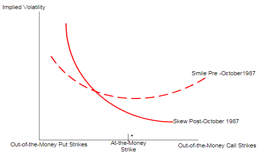
Figure 3: CBOE skewness index

This skew can indicate panic in the market. If the implied volatility of a put option is much higher than the call option, this can be explained by the fact that the ratio of hedges made by investors to avoiding downside risks is not one.

In the example of Figure 3, the chart shows that the S&P 500 index exhibits a negative volatility skew. One reason is that more and more investors like to buy stock-price call options instead of buying stocks directly, because buying options can bring leverage, that is, paying an option premium equivalent to a part of the stock price can enjoy the same stock price. The benefits of the increase, while buying stocks need to take up the equivalent of 100% of the stock price. The result of this is that the investor's rate of return will increase, so the market's demand for call options within the stock price increases, and the implied volatility level of the call option with lower strike prices rises.

Therefore, although the normal distribution curve of the Black-Scholes model gives equal probability at both ends, the stock option market tends to behave more pessimistically. Interestingly, the bitcoin market is much more optimistic than it is.

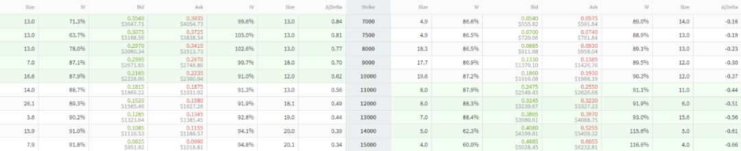
Figure 4: Bitcoin option table with maturity date of December 27, 2019

Figure 4 shows the Bitcoin derivatives that expired on December 27, 2019 by the Bitcoin option platform Deribit. It can be seen that the two prices (7,000 and 13000) that deviate from the current price of Bitcoin (10000+) show different implied volatility: implied volatility of puts bought at 7000 (right) The rate (IV) is 86.6%, while the 13,000 point call option (left) has a slightly higher IV of 90.2%. This suggests that the value of the out-of-the-money put option is much lower than the out-of-the-money call option. Although this option list does not represent the entire bitcoin option market, it also indicates that a significant number of speculators/investors underestimate the downside risk.

Therefore, the Black-Scholes model cannot be deified. On the contrary, when using this model to price options, it should retain a skeptical attitude. As pointed out above, the Black-Scholes model is still widely used. It provides more benchmarks. Traders can quickly find the relative price of options, but at the same time some platforms overproduce this easy-to-apply model. rely.

Unpredictability of kurtosis

 

The kurtosis is the flatness of the data distribution. The large data distribution at the tail has a large kurtosis value, reflecting the risk characteristics of the tail at the future. The sample excess kurtosis formula is:

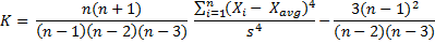
among them:

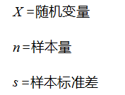
The kurtosis is:

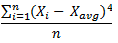
In calculating the kurtosis of the asset's return distribution, it is necessary to deviate from the mean (the difference between each random variable) X and the average of all values). This deviation can be expressed as:

In statistics, the moment describes the shape of the probability distribution. In general, the first and second moments represent the mean and variance of the distribution, respectively, and the third moment represents the skewness. As mentioned earlier, skewness is a measure of how asymmetric or skewed the distribution is. The fourth step reflects the sharpness of the distribution and changes the curve of the normal distribution in different ways. It can be expressed as:

In order to eliminate the influence of variable value levels and unit of measurement, the fourth step of the central moment is used in practice. The ratio of the ratio is used as an indicator of kurtosis, called the kurtosis coefficient. When calculating kurtosis, it is generally assumed that excess kurtosis has been taken into account. The kurtosis of the normal distribution is 3, as shown in Figure 5. If the kurtosis of a distribution is greater than 3, it is called the positive kurtosis (spike leptokurtic). From the morphological point of view, it is steeper or more tail than the normal distribution. Thicker, that is, the range of values ​​on both sides of the mean will be larger than the normal distribution, which means that the asset price will become more unpredictable because the probability of price volatility increases; when the kurtosis is less than 3, the negative peak Degree (flatkurtic), in terms of morphology, is more gradual than the normal distribution or thinner at the tail.

When calculating the excess kurtosis, the formula is: excess kurtosis = kurtosis -3. When an asset has an excess kurtosis, the inherent risk of holding the asset is greater.

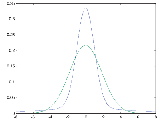
Figure 5: Normal distribution with the same variance and shape of positive kurtosis

The kurtosis can be used to measure risk, and here we temporarily ignore the basic assumption of "random walk". Finding the kurtosis of the rate of return within any given time frame allows investors to understand how volatility is distributed. The normal distribution of return on assets can describe different risk situations. Most people in the investment community choose to regard volatility and risk as one thing. The greater the volatility of assets, the greater the risk. Conversely, the smaller the asset volatility, the safer it is. However, this duality of volatility/risk ignores the nature of volatility and even attributes the benefits of a normal distribution to the “risk” category.

When we limit the income to a normal distribution, then the probability of different income situations is known. For example, assuming that the normal distribution edge of an asset's return reaches -50% and 50%, such an asset would be considered extremely unstable, but if the benefit is normally distributed, then the curve can be derived The tail and edges have 2 and 3 standard deviations, respectively, compared to the mean. Once this information is known, the investment strategy can be adjusted around this possibility, and even very unstable assets can be traded like less volatile assets. Therefore, rather than confusing risk and volatility, let them establish orthogonal relationships, which can be used as a risk risk compass.

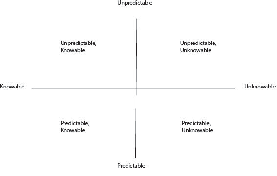
Figure 6: Orthogonal relationship between volatility and risk

In Fig. 6, it is assumed that the vertical axis is the predictability of the price, and the horizontal axis is the known degree of the probability distribution of the return. In this picture, the upper quadrant is an unpredictable price, which stands for “random walk”; the left quadrant is the probability distribution of the yield, and the return is a normal distribution.

In Figure 7, the upper left corner represents the assets in the Black-Scholes model based on the "ideal" assumption. Such assets undergo a "random walk", the price is unpredictable, and the rate of return is normally distributed, so the probability distribution is known. The lower right corner represents the opposite of the Black-Scholes model. The price of the asset is predictable, but the probability distribution is unknown. This asset can be considered manipulated, whether through insider trading or technical analysis in general, the price is It is completely predictable, but the probability of occurrence is uncertain. Over time, the price of such an asset can be fully manipulated, and there is no need to predict the probability distribution of the rate of return. The price in the lower left corner is predictable, and the probability is also known. Such assets can be considered “stable” and there should be no price deviations, and future yields are also known. Finally, the upper right corner represents the assets that follow the “random walk”, but the distribution of the probability of return is not normal.

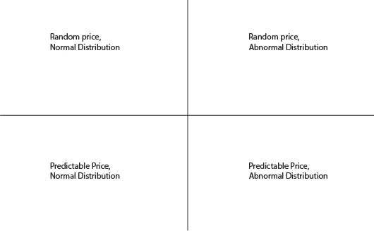
Figure 7: Volatility – Risk Compass

With the volatility-risk compass, you can portray clearer images to clarify the risk profile of an asset. On this basis, kurtosis can be used to determine which quadrant an asset falls into. The peak of the asset measures the risk of the option because the excess kurtosis means that the pricing by the Black-Scholes model is not necessarily reliable.

In addition, when studying “risk-adjusted returns,” finding the kurtosis of assets in a portfolio can more accurately measure the value of the portfolio. This is because kurtosis can measure the “tail risk” of a portfolio. By identifying “tail risks” rather than just considering volatility, investors can better clarify the risks in their portfolios. Therefore, when trying to explain the risks of Bitcoin, it is not enough to focus solely on the volatility of Bitcoin. Assuming that the rate of return follows a normal distribution, the exact price of the bitcoin option can be given to quantify the risk. And if the rate of return does not follow a normal distribution, then the probability of the distribution of returns on the option price becomes less informative.

Bitcoin kurtosis

 

By observing the daily yield of Bitcoin from 2016 to 2019 (data source: coinmarketcap), you can get the excess kurtosis of Bitcoin. Since January 2016, Bitcoin has experienced excessive kurtosis.

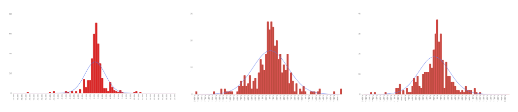
Figure 8: Bitcoin Daily Revenue 2016 (left), 2017 (middle), 2018 (right)

Figure 8 shows the distribution of Bitcoin daily returns for 2016, 2017, and 2018, and plots the normal distribution curve based on the data. It is clear from the chart that Bitcoin does not follow a normal distribution. Comparing Figure 8 with Figure 5, we can see that Bitcoin is more like a positive kurtosis. After calculating the excess kurtosis in 2016, 2017, and 2018 (10.03, 3.29, and 2.05, respectively), the daily yield for each chart ranges from -20.00% to 20.00%. But in 2017, two observations (22%) exceeded this range. For Bitcoin, 2017 is a particularly unstable year. Bitcoin volatility declined slightly in 2018, but there is still a significant “tail risk”. It is worth noting that bitcoin prices have seen a more dramatic decline in 2018.

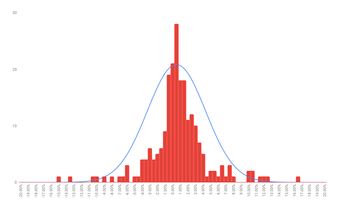
Figure 9: Bitcoin daily earnings in 2019

So far (September 2019), the kurtosis of Bitcoin has not declined. On the contrary, compared with a slight increase in 2018, the excess kurtosis is 3.92. Although the daily income in this year has a large probability distribution close to its average value, the probability distribution at the tail is relatively uniform. This shows a classic positive kurtosis with a thicker tail and a range of values ​​on both sides of the mean greater than the normal distribution.

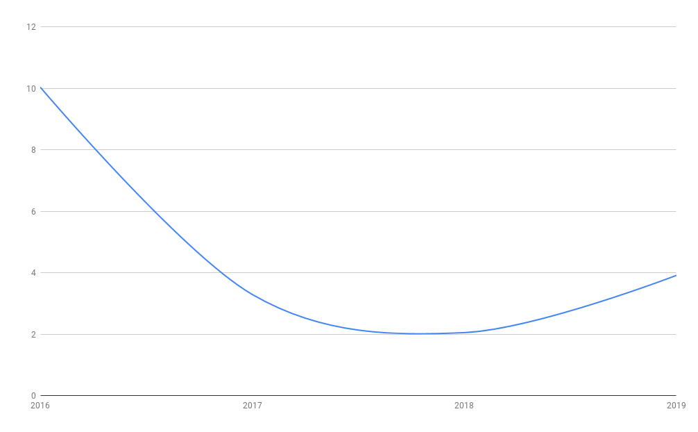
Figure 10: 2016-2019 Bitcoin excess kurtosis

Overall, the excess kurtosis shows that the probability skew of the bitcoin daily rate of return using the Black-Scholes model yields an average and tail that will be larger than expected. Pricing options can become very difficult because implied volatility becomes less reliable. Excess kurtosis means that most of the price changes become unpredictable and volatility does not follow a normal distribution.

As a result, an asset may exhibit relatively low volatility, and thus the probability of a large price change is low, but such volatility does not really represent the volatility of an asset. Looking back at the volatility-risk compass in Figure 7, Bitcoin is probably the type of asset represented in the upper right corner. It is speculated that the price of Bitcoin is unpredictable and random, and the probability of its return does not obey the normal distribution.

Comparison and conclusion

 

So far, we have proven that Bitcoin behaves as an excess kurtosis. Is Bitcoin an outlier compared to the more widely discussed stock market? Also, no. In addition to Bitcoin, there are many assets that also show excess kurtosis, even the S&P 500 (S&P 500 Index). In 2018, the S&P500 showed an excess kurtosis of 3.09. Below the excess kurtosis of Bitcoin 2016, 2017 and 2019, but higher than 2018. For the S&P500, 2018 was a very unstable year, and the stock market experienced a sharp rise and fall. As shown in Figure 11, at the beginning of 2018, the index suddenly fell more than 10%, corresponding to the relatively extreme kurtosis.

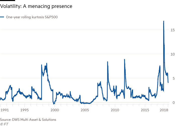
Figure 11: S&P 500 kurtosis changes (Source: Financial Times)

In the histogram of Figure 12, the daily yield distribution of the S&P 500 is closer to a normal distribution than Bitcoin. Although some of the daily gains far exceed the normal distribution curve, there is a clear excess kurtosis. But in general, only 6 of the 250 observations of the S&P500 exceeded the normal distribution curve. Of the 364 observations of the Bitcoin daily yield in 2017, 28 exceeded the normal distribution curve. Based on the data comparison, we find that the S&P500 daily yield curve declines very fast, and the possibility of extreme price fluctuations is low, making it difficult to predict extreme changes in events, and the fluctuations are unpredictable.

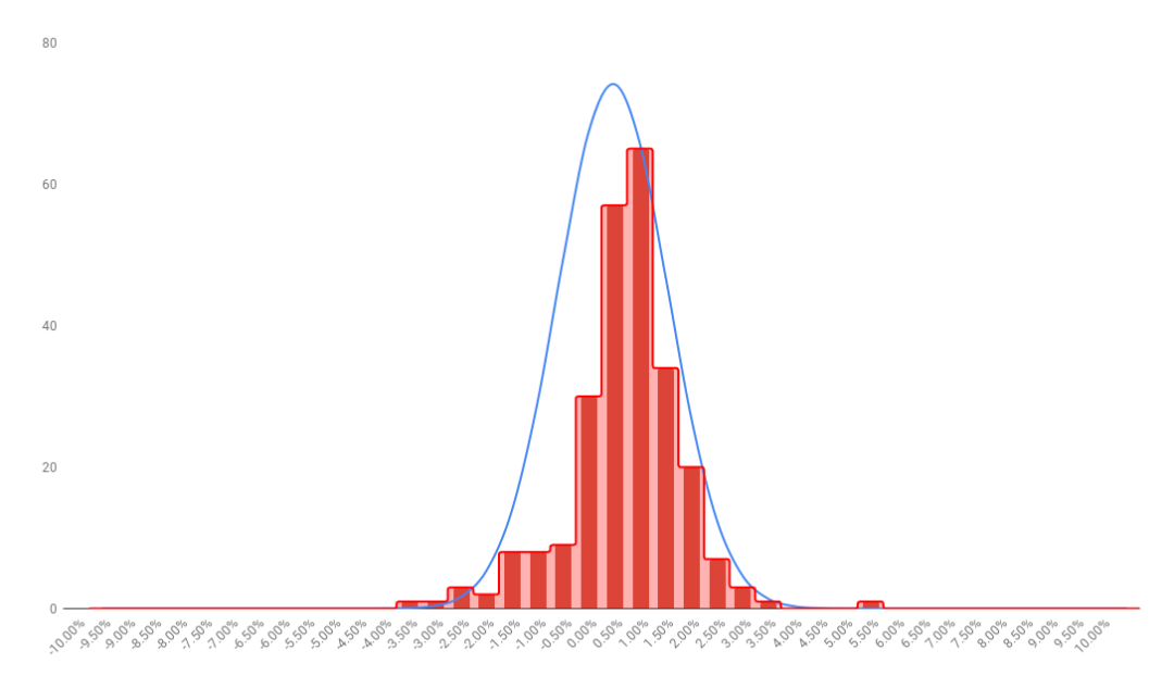Figure 12: Standard & Poor's 500-day yield in 2018

So what can we get from it? Although the S&P 500 does not fall into the normal distribution curve, it does have a more normal distribution curve than Bitcoin. The specific reasons for this result have yet to be scrutinized, but I think there are at least three possibilities. First, Bitcoin represents different asset classes and follows different basic assumptions than the broader stock market. Second, the current bitcoin market is still immature and lacks the control of a specialized investment institution. Third, in general, the reliability of the Black-Scholes model is questionable, and the unpredictability of fluctuations becomes the "new normal."

Regardless of which of these reasons, we can conclude that in this case, the bitcoin option pricing model is likely to be wrong, and the “triangular arbitrage” valuation of the Bitcoin portfolio is not accurate. Especially in the case of many new cryptocurrency derivatives exchanges, the latter may lead to more problems, because the relatively high implied volatility of Bitcoin and the excess peaks behind this volatility Degrees will greatly reduce the ability of investors to avoid risks and cannot quantify risks.

Note

From Brenner and Subrahmanyan's "Simple Formula for Calculating Implicit Standard Deviation" and the Black-Scholes model we can get:

among them:

In our first example of corn, the option price was $2 and the current corn price was $3.5, and the option contract was assumed to last for six months. It is worth noting here that the above formula is to calculate the volatility of the call option price. And this corn example is a put option. Therefore, the volatility calculated from this formula will be slightly inaccurate. However, for the sake of simplicity, we treat this option as a call option.

Use the above formula to get:

σ=√(2π/5)*(2/3.5)

σ=202.73%

Source: Brenner, Menachem and Marti Subrahmanyan, “A Simple Formula to Compute the Implied Standard Deviation.” Financial Analysts Journal 44(5) (1988). 81

Reference material

[1] Black, Fischer & Myron Scholes. “The Pricing of Options and Corporate Liabilities.” Journal of Political Economy 81(3) (1973).

[2] Fama, Eugene F. “Efficient Capital Markets: A review of Theory and Empirical Work.” The Journal of Finance 25(2) (1970).

[3] Hull, John C. Options, Futures, and Other Derivatives. Tenth Edition. New York: Pearson Education, (2018).

[4] MacKenzie, Donald. An Engine, Not a Camera. Cambridge, MA: MIT Press, 2006.

McAlevey, Lynn G. and Alan F. Stent. “Kurtosis: a Forgotten Moment.” International Journal of Mathematical Education in Science and Technology 49(1) (2017).

[5] Malkiel, Burton G. “The Efficient Market Hypothesis and Its Critics.” Journal of Economic Perspectives 17(1) (2003).

[6] Westfall, Peter H. “Kurtosis as Peakedness, 1905–2014. RIP” Am Stat 68(3) (2014).

Article source: Hash

Original: Kurtosis and Bitcoin: A Quantitative Analysis

Translator: Adeline

We will continue to update Blocking; if you have any questions or suggestions, please contact us!