From parameter A, examining the technical details and governance philosophy of Curve

Examining Curve's technical details and governance philosophy based on parameter A

A year ago, I spent some time participating in Uni V3 LP and had a great time. Around the same time, there was a notion that being an LP in the Curve Tricrypto Pool was a stable and popular asset allocation method for generating continuous profits. This attracted me to read the Curve V2 whitepaper. I developed a vague understanding of the characteristics of Uni and Curve, and realized that they had significant differences. Uni pursues a free market as much as possible, while Curve has a more planned and precise economic approach.

To further explore this concept, it was necessary to thoroughly understand the technical details of Curve V2. So, a few months ago, I began to carefully study Curve V2. As the founder of Curve and a former researcher in the field of physics, Michael effortlessly combines mathematical formulas in the whitepaper. As a reader with limited mathematical knowledge, I struggled to grasp the core and less intuitive elements, such as Xcp and its related components, D and Virtual Price.

During the research process, I also realized that even for experts, mastering Curve V2 is not something that can be achieved overnight. Curve V2 is a more complex and generalized version built upon V1. To better understand the design essence, it is important to first understand Curve V1. It’s like retracing the steps of the experts.

In V1, the main characters are A and D. The parameter A may seem simple, the larger the value of A, the more liquidity is allocated around price 1. This can be summarized in a single sentence. However, when reviewing the records from that time (Discord/governance forums/Telegram), various issues related to A constantly came up, including technical aspects and protocol governance. These discussions were diverse and rich in content, which led to the writing of a dedicated section about the A parameter. The following is a part of it: First, it discusses the influence of A as a unique parameter for a single DEX on the entire market. Managing an influential parameter becomes an important issue, and the subsequent section further explores the technical details of regulating A.

• LianGuai Daily | Flashbots raises $60 million in funding; Anthropic, Google, Microsoft, and OpenAI launch cutting-edge model forum.
• Vitalik Buterin Proof of Personhood based on biometric identification is more effective in the short term, but technology based on social graph is more robust in the long term.
• Ethereum Foundation’s 10th AMA Highlights Validator Set, Randomness, DVT, and Technical Direction

While delving into the microscopic details of the A parameter, I have not forgotten the original intention and the initial interest in comparing the characteristics of Uni and Curve. I often find myself questioning whether these details reveal a fundamental difference in ideology.

1. The relationship between the A parameter and the overall market price

On September 4, 2020, Andre Cronje posted a proposal on the Curve governance forum, suggesting adjusting the A parameter of the y Pool from 2000 to 1000. This sparked a small amount of discussion and some opposing opinions, but a few days later, it was calmly approved through voting. At first glance, it seemed like a topic of little significance compared to the extensive debates on certain issues in many DeFi projects later on, and it didn’t seem worth mentioning.

It is precisely the mathematical complexity of Curve that raises the threshold for discussions, concealing the importance of certain issues and even hindering a true understanding of Curve’s essence. This series of articles focuses on the A parameter, going back to ancient times, examining several historical events, and attempting to simplify the mathematics to reveal some truly important propositions about Curve. This article is the first one, starting with this proposal by AC.

Can parameter A affect market prices?

Statements from AC and the opposition

Returning to AC’s proposal, in late August and early September, the yETH vault expanded rapidly (the operation of the yETH vault involves depositing ETH, minting DAI, depositing it into the yDAI vault, which then deposits it into the Curve y Pool to earn CRV rewards, sell them for ETH, and ultimately achieve ETH-based returns).

Unfortunately, this coincided with a rapid decline in ETH prices, which increased the demand for DAI. The share of DAI in the y Pool decreased rapidly, reaching as low as 2%.

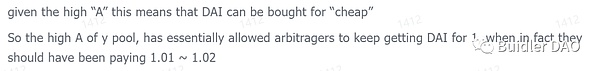
AC believes that the A parameter of the y Pool is too high (A = 2000), resulting in the y Pool supplying DAI to the market at a price that should not be so cheap. For example, they make the following argument:

The opposition mainly revolves around two perspectives, one of which is related to the selling pressure caused by continuous CRV sales from the yETH vault, which will not be discussed here.

What interests me is another perspective related to the price determination mechanism.

For example, @iamaloop’s opinion is that there is no such thing as Cheap DAI, as arbitrageurs will equalize prices everywhere. The A parameter can only affect the imbalance of the percentage of different coins in the Curve y Pool when the coin price is equal to the market price.

@sjlee expresses a similar view. @angelangel0v points out that arbitrageurs cannot obtain lower prices just because of a high A parameter.

In summary, the opinions of these three individuals are: the price of DAI is determined by market supply and demand, and the A parameter can only determine the depth of the Curve y Pool at different DAI price points and cannot determine the market price.

The confrontation of these two viewpoints actually raises a question: what is the relationship between the A parameter and market supply and demand?

The important impact of the A parameter on the supply side

In certain situations, the A parameter has an extremely significant impact on the supply side, making it one of the most important variables in price determination.

Before discussing the supply and demand curve, let’s first discuss some important assumptions and basic factors.

First, Curve operates on the LianGuaissive LP model. In my opinion, as the supplier, LianGuaissive LP is relatively stable, meaning that its frequency of operations is relatively low when faced with changing market conditions (by “operations,” I mean balancing liquidity deposits and withdrawals, or accessing liquidity in single-coin mode with trading attributes; “relatively” refers to the fact that it is compared to Uni V3’s actively managed LP or CEX’s market makers).

Second, a large portion of Curve LP’s earnings come from CRV token rewards that are not closely related to transaction fees, especially in 2020, and the absolute return rate is high. Therefore, when facing relatively small market changes (e.g., 1-2%), LPs are more stable.

The combined effect of the above two points is that Curve LP is more stable.

Third, for certain tokens, Curve is the largest liquidity pool. For example, in 2020, the y Pool was the largest exchange pool for DAI.

If all three of the above points hold true, the supply curve of the entire market will be primarily determined by the Curve Pool. Remembering these three premises, we will now enter into a discussion on the supply and demand curve.

Let’s first look at the supply curve of the entire market, where the A value affects the shape of the curve. The higher the A value, the flatter and longer the curve near the price of 1, indicating greater liquidity.

Market-wide supply and demand curve graph

Now let’s look at the demand curve. Let’s assume a stable market condition – demand curve 1. When ETH experiences a sharp decline, the demand for closing CDPs sharply rises, and the market needs more DAI. As a result, the demand curve shifts to the right – demand curve 2.

By observing the intersection of the supply and demand curves, we can clearly see the impact of the A parameter on the price. The lower the A value, the higher the corresponding new equilibrium price.

Therefore, if a token’s primary liquidity is in Curve, the A parameter has a significant influence on price determination.

Conclusion

The A parameter more or less affects the price determination of the entire market, the extent of which depends on factors such as the token reward scale of the Curve Pool and the market share of the Curve Pool.

As such an important parameter, it naturally gives rise to a series of questions. What is the mechanism for setting the A parameter? Who sets it and what are the criteria for choosing the value?

Furthermore, the market is not static, which leads to a series of dynamic questions. When does the A parameter need to be adjusted? What impact does adjusting the A parameter have on the AMM formula? And so on.

II. Changes and gains/losses brought about by adjusting A

As of April 17, 2020, over a month has passed since 312, but DAI is still in a positive deviation state, with a price of around 1.02.

Michael (founder of Curve) initiated a poll on Twitter to see if people supported adjusting the A parameter of the Compound pool from 900 to 400.

49 people participated in the poll, but there was only one respondent. After 8 hours, Michael adjusted the A parameter to 400 and tweeted again, with 0 replies.

At that moment, very few people were actually able to participate in the discussion on this issue. Michael was probably immersed in his own experiment, adjusting parameters, observing, and improving. In the snippets of conversation on Telegram, I could sense his enthusiasm and enjoyment.

Regarding this adjustment of the A parameter, it resulted in a daily loss of about 0.1%.

The purpose of this article is to clarify what it means when A is adjusted and why it leads to losses.

An illustration of curves corresponding to different A values

I have selected a set of actual parameter settings to present in a graph. The discussion in this article is focused on Curve V1 Pool, as outlined in the V1 whitepaper.

The parameters corresponding to the black curve are: A = 10, D = 20,000.

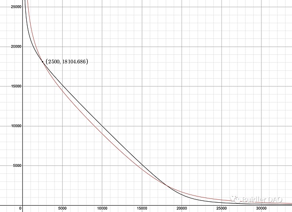
The current pool is at the black dot, with the quantities of X_token and Y_token being 2500/18105 respectively, and the price is approximately 1X_token = 1.36 Y_token.

At this moment, if A is reduced to 3, the curve will become a red line. The parameters of this curve are: A = 3, D = 19,022.

Comparing the red and black curves, it is clear that the black curve has a higher proportion of approaching straight lines, which is also the core function of A. The larger the A, the more liquidity there is around the price of 1; the A value of the black curve (10) is higher than that of the red curve (3). Correspondingly, the liquidity in the range away from the price of 1 is greater in the red curve than in the black curve.

At the time of the Twitter poll, DAI was slightly off-peg. If the red curve with a low A value is used, it can provide more liquidity than the black curve with a high A value. This is also why Michael wants to adjust A, he hopes that the pool can capture more fees.

Let’s go back to the changes brought by reducing A to 3. At the moment of reducing it to 3, the quantities of the two tokens in the pool did not change, but the D value changed. In addition, it can also be seen from the graph that the slope of the tangent line at the current point has changed, and the shape of the curve has also changed.

The following specifically discusses these changes. If we look at the changes in the slope of the tangent line and the shape of the curve from a different perspective, it will be more intuitive. The change in D value involves the topic of pool profit and loss evaluation.

Changes after adjusting the A value from the perspective of the order book

The Curve pool can be understood from the perspective of the order book. For a single pool, depending on its A and D parameters, it corresponds to different distributions of order quantities at all price points, and all orders are interdependent and exist as a whole.

In the previous case, when A dropped from 10 to 3, it can be understood as a comprehensive adjustment of all orders, transforming from a set of black orders to a set of red orders.

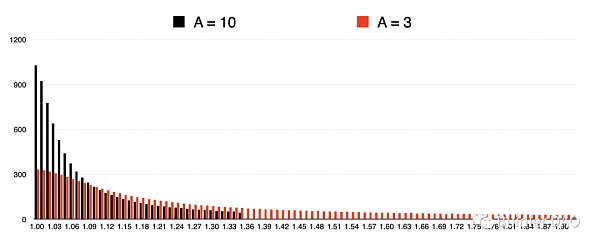
Let’s start with some basic explanations for the above figure.

The horizontal axis represents the price, where 1.00 represents 1 X_token = [1.00 ~ 1.01) Y_token, 1.01 represents 1 X_token = [1.01 ~ 1.02) Y_token, and so on. In order to save space, I have omitted the orders with prices less than 1.00.

The vertical axis represents the quantity of Y_token (i.e., the buy orders for X_token). The black part has no data in the price range above 1.36, because the current price on the black curve is 1.36, and prices above 1.36 represent higher-priced sell orders for X_token. This graph only examines the part where Y_token is used for buy orders, so there is no data for the part above 1.36.

Let’s look at the comparison between black and red. First, the current price has changed, corresponding to the change in the slope of the tangent line mentioned in the previous section. After A is adjusted, the current price instantly changes to 1.92, and the red part of the orders extends to 1.92. This means that a certain quantity of Y_token has been placed in batches as buy orders for X_token in the price range of 1.36 – 1.92.

This is actually a strange change, the current price of a DEX has changed without any swaps. We can immediately think that this will create a spread with the market price, and we assume that arbitrageurs will instantly intervene to bring the price down to 1.36.

In addition, it can be seen that the number of orders at each price point from 1.00 to 1.36 is different, overall, there are more orders at the higher prices. This corresponds to the changes in the shape of the curve mentioned in the previous section.

Profit and Loss from A Adjustment – The most direct calculation method

Michael’s suggestion mentioned that lowering the parameters of Compound Pool A would result in some losses (‘Wipe One Day’s Profits’). Before discussing the mathematical relationship behind this, it is necessary to define “loss/profit” clearly.

According to the most direct idea, defining profit and loss is simple. Convert the value of the two tokens into U or either one of them (X_token or Y_token), from two dimensions to one dimension, and then compare the total value before and after the A adjustment. This is also what Michael mentioned as ‘With Impermanent Loss’.

Let’s briefly discuss this concept of profit and loss. For the sake of simplification, let’s assume that the transaction fee is 0.

Based on the example we have been using, after A is lowered, the instantaneous price of X_token becomes higher, and arbitrageurs intervene to bring the price back to the level before the A adjustment, which will result in losses. The reason is simple. As mentioned in the previous section, after A is lowered, it is equivalent to placing many buy orders for X_token at a price higher than the market price. These abnormal buy orders are capitalized by arbitrageurs, which will inevitably result in losses.

It will be clearer from the curve graph.

The black dots and black curve represent the state of the pool before the adjustment, corresponding to a price of 1.36. After A is lowered, the pool operates along the red curve. At the moment of the adjustment, the pool price becomes 1.92, and arbitrageurs quickly move the state of the pool from the black dot to the red dot, corresponding to a price of 1.36.

It is necessary to compare the total value of the pool before and after the A adjustment, and the method is relatively simple.

First, look at the total value after the A adjustment (after arbitrageurs intervene). Find the intersection of the tangent line at the red dot on the red curve and the Y-axis, which represents the amount of the two tokens converted into a single Y_token at the current price.

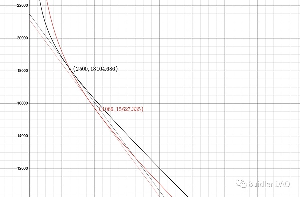
Then, look at the total value before the A adjustment. Find the intersection of the tangent line at the black dot on the black curve and the Y-axis. Because the prices before and after the A adjustment are the same (after arbitrageurs intervene), this tangent line is parallel to the tangent line in the first step.

Obviously, the intersection of the black tangent line and the Y-axis is higher, which means the total value before the A adjustment is higher. The A adjustment has caused a loss in the total value.

The above discussion is limited to the instantaneous loss after A is lowered, which is relatively simple. However, if we extend the tracking time and explore the long-term profit and loss brought by the A adjustment under different price trends, it becomes somewhat complicated. This depends on whether the price moves towards a more unanchored direction or returns to perfect anchoring. The total value after the A adjustment may be lower than the state without adjusting A, or it may be higher. This will not be further elaborated here. The purpose of this article is only to briefly demonstrate how the A adjustment affects the total value of the pool, without seeking a comprehensive system discussion.

Eliminating Impermanent Loss Evaluation

Converting based on the current prices of the two tokens, taking impermanent loss into account, is the most intuitive measurement method, but it is more complicated. Curve introduces another unique method of evaluating losses and gains, which eliminates the factor of impermanent loss and simplifies the calculation, making it applicable in most cases.

This is the D value, which is another core parameter of the Curve formula outside of A. The Virtual Price we see in each pool on the Curve official website is calculated based on the D value.

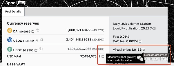
The D value is the total quantity of the two tokens in the pool when the pool price is 1 (perfectly anchored). Since the price is 1 at this moment, the quantities of the two tokens can be simply added together. The point where the pool price is equal to 1 is the intersection of the curve and the line x=y.

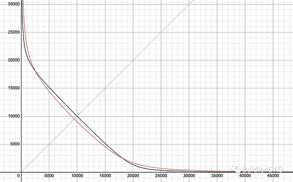
Returning to the previous example, it is obvious that the D value becomes smaller after A is adjusted downwards. Therefore, in the long run, if the price can be restored to its anchor, the change in the D value can reflect the loss caused by the adjustment of A.

In the example I used earlier, the current price is 1.36, which is actually an extreme case. For Curve V1-like pools, such as mainstream stablecoin/LSD pools, the price will not deviate too much from 1. When the price is close to 1, the impact of impermanent loss is small, so the change in the D value can be directly used to approximate the evaluation of losses and gains.

The D value, as a one-dimensional measurement and one of the parameters of the pool, is easy to calculate and track historical values, making it suitable for approximate evaluation of losses and gains.

Conclusion

The adjustment of the A parameter is equivalent to a rearrangement of the orders on all price points of the order book, changing the current price point, changing the D value, and resulting in losses and gains.

Therefore, a one-time large-scale adjustment of the A parameter gives a sense of abruptness and even a sense of flaw. The whitepaper does not involve dynamic management of A, perhaps because Michael gradually realized the need to revise the adjustment method for the A parameter after Curve was launched and operated for a period of time. Under the tweet announcing the completion of the Compound Pool A parameter adjustment, Michael added a comment. In subsequent versions of the pool, the adjustment of the A parameter was changed to a gradual completion over a period of time.

Is the one-time adjustment method of the A parameter in the old pool just a flaw? It’s not that simple. Behind it, there is also a hidden vulnerable point. Fortunately, it was discovered by a white hat hacker (the depth of understanding of the protocol is truly extraordinary). A separate article will be written later to discuss this attack method.

We will continue to update Blocking; if you have any questions or suggestions, please contact us!