Technical Primer | Zk-stark: Low Degree Testing

Foreword

The second article in this series, using supermarket receipts as an example, described the specific process of Arithmetization. This article will be based on another example, while reviewing the Arithmetization process, the content will be extended to the polynomial LDT process.

New instance

Alice Claim: "I have 1000,000 numbers and they are all in the range [0,9]". In order to facilitate the verification of the verifier Bob, Alice first needs to perform Arithmetization transformation on Claim. The process is shown in Figure 1 below (in the figure: the black arrow represents the main flow, the red arrow represents additional explanatory information, and the yellow circle corresponds to the index detailed below)

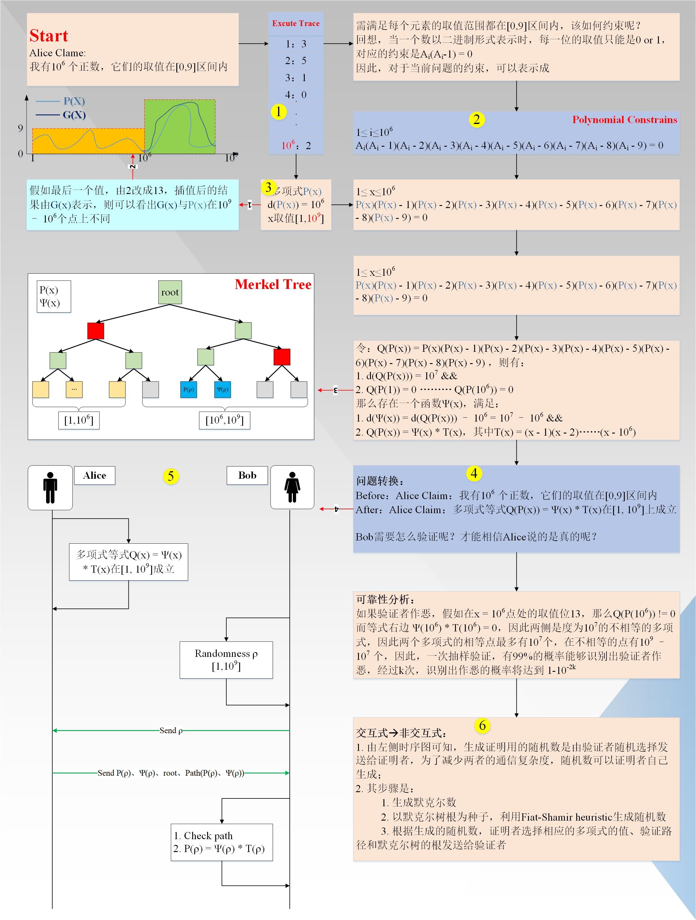
The following details the corresponding process:

• Expansion of Layer0 layer to be the CDN of the blockchain
• Proficient in Filecoin: Hello protocol of Filecoin source code
• Getting started with blockchain | What can blockchain do in agriculture?

1. First, the execution trace (EXCUTE TRACE) is generated. In fact, it is a table with a total of 1000,000 rows (in fact, in order to achieve the purpose of zero knowledge, some random values ​​need to be added after the execution trace. The specific number is The prover and verifier are coordinated and decided, as an extension, not specifically described);
2. Generate polynomial constraints (Polynomial Constrains), polynomial constraints satisfy each line of the execution trajectory (personal understanding: step 1, 2 does not have a certain sequential dependency relationship, but it is customary to generate the execution trajectory first, then generate the constraint polynomial);
3. Interpolate the execution trajectory to obtain a polynomial P (x) with a degree less than 1000,000, and the value of x is [1,1000,000], and calculate the value at more points. The value range of x is expanded to [1,1000 , 000,000] (Reed-Solomen system coding); if the prover has a value that is not in the range of [0,9] (shown by red line 1/2 in the figure), if it is the 1000,000th point, its actual value It is 13, greater than 9, and the curve G (x) after interpolation is shown in the figure. In the figure, P (x) is a valid curve and G (x) is an invalid curve. It can be seen that the two curves have a maximum of 1,000,000 intersections in the range of the value of the variable x [1,1000,000,000], that is, 1000,000,000-1000,000 points are different, which is very important.
4. Combine the interpolated polynomials P (x) and polynomial constraints to transform them into the final form:

Q (P (x)) = Ψ (x) * T (x), where T (x) = (x-1) (x-2) … (x-1000,000), x takes the value [1, 1000,000,000]

Where d (Q (P (x))) = 10,000,000, d (Ψ (x)) = 10,000,000-1000,000, and d (T (x)) = 1000,000;

1. At this point, the problem turns into a problem where Alice claims that "the polynomial equation holds within the range of the value of the variable x [1,1000,000,000]". So how does the verifier Bob verify? The specific process is as follows (shown as red line 3/4 in the figure):
   1. The prover Alice calculates the values ​​of the polynomials P (x) and Ψ (x) at all points locally, yes! From 1 to 1000,000,000 and form a Merkel tree;
   2. The verifier Bob randomly selects a value ρ from [1,1000,000,000] and sends it to the prover Alice, asking him to return the corresponding information (in fact, in order to achieve the purpose of zero knowledge, only from [1000,000, 1000,000,000] randomly select a point);
   3. The prover Alice returns P (ρ), Ψ (ρ), root, AuthorizedPath (P (ρ), Ψ (ρ)) to the verifier Bob;
   4. The verifier Bob first verifies the validity of the path verification values ​​P (ρ) and Ψ (ρ) according to the Merkel tree, and then the equation Q (P (ρ)) = Ψ (ρ) * T (ρ), if true, The verification is passed;

Completeness analysis: If the verifier Alice is honest, then the equation Q (P (x)) must be divisible by the target polynomial T (x), so there must be a d (Ψ (x)) = d (Q (P (x)))-d (T (x)) polynomial Ψ (x) satisfies Q (P (x)) = Ψ (x) * T (x), so for any x, the value is in [1 , 1000,000,000], the equation will hold;

Reliability analysis: If the verifier Alice is dishonest, that is, similar to the assumption in step 3, on x = 1000,000, the value of P (x) is 13, then Q (P (1000,000)) ! = 0, but on the right side of the equation, T (1000,000) = 0, so Q (P (x))! = Ψ (x) * T (x), that is, the two sides of the equation are not equal polynomials, and their intersections There is a maximum of 10,000,000, so the probability of passing the verification by only one random selection is only 10,000,000 / 1000,000,000 = 1/100 = 0.01. After k times of verification, the probability of passing the verification is only 1- 10 (^-2k) ;

1. The above verification process is interactive. If it is non-interactive, you can use Fiat-Shamir heuristic to transform and use the root of the Merkel tree as a random source to generate random points to be queried.

LDT

We ignore an attack method, that is, for each number x, the prover randomly generates p, and then according to Ψ (x) = Q (p) / T (x), these points are not at any degree less than 1000,000. Polynomial, but can be verified by the verifier. As shown in Figure 2:

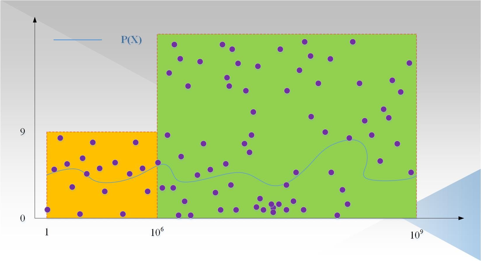
In the picture: The purple points are randomly generated points p. These points have a high probability that they are not on a polynomial with a degree less than 1000,000 (in fact, the first 1000,000 points can be disregarded, because the verifier will only start with 000, 1000,000,000]. Because even if 1000,000 points are selected to interpolate a polynomial with a degree less than 1000,000, other points cannot be guaranteed to be on this polynomial, because other points are randomly generated. Therefore, a way is needed to ensure that the degree of the prover P (x) is less than 1000,000, and the degree of Ψ (x) is less than 10,000,000-1000,000. This is the goal of LDT. What is the specific process of LDT? please watch the following part.

For example, if Alice wants to prove that the degree of the polynomial f (x) is less than 3, it may be 2 or 1 degree. The general process is as follows:

1. The verifier Bob randomly selects three values ​​a, b, and c and sends it to the prover Alice;
2. The prover Alice returns f (a), f (b), f (c);
3. The verifier Bob interpolates a polynomial g (x) with a degree less than 3, and then randomly selects a point d and sends it to the prover;
4. The prover Alice returns f (d);
5. The verifier Bob compares the values ​​of f (d) and g (d), and if they are equal, it proves to be true.

Returning to the general situation, the process can be represented by the following figure 3:

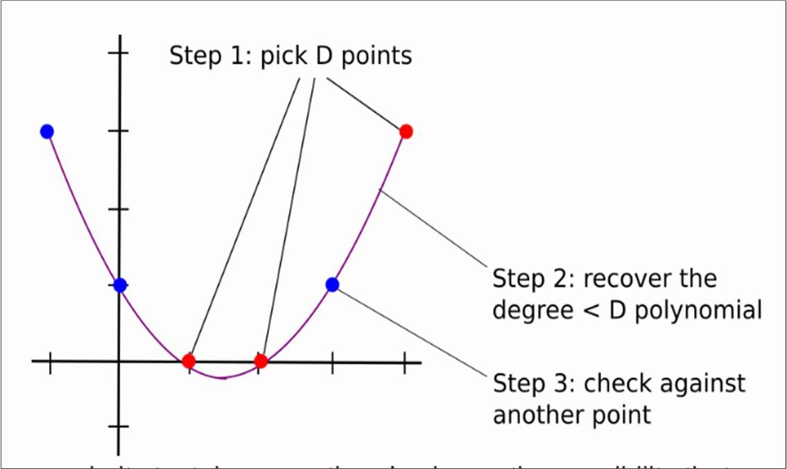
It can be seen that if D is large, the number of interactions between Alice and Bob is D + k, and the complexity is high; is there a way to make the number of interactions between the two less than D, making the verifier I believe that the degree of the polynomial is less than D, and it is definitely impossible to directly return less than D points, because it cannot uniquely determine a polynomial with a degree less than D, so the prover needs to send some auxiliary information. Below we take P (x) as an example to elaborate this process (in fact, it should be proved that the linear combination of P (x) and Ψ (x) is less than 10,000,000-1000,000. This article focuses on LDT, so only P (x x) as an example, this does not affect the understanding of LDT).

1. If P (x) = x + x ^ 999 + x ^ 1001 + x ^ 999999 = x + x ^ 999 + x * x ^ 1000 + x ^ 999 * (x ^ 1000) ^ 999;
2. At this point, we find a two-dimensional polynomial G (x, y) with values ​​ranging from [0, 999999999] and [01000, 9999999991000], which satisfy:
   1. G (x, y) = x + x ^ 999 + x * y + x ^ 999 * y ^ 999 It can be found that when y = x ^ 1000, it satisfies:
   2. G (x, y) = G (x, x ^ 1000) = x + x ^ 999 + x * x ^ 1000 + x999 * (x ^ 1000) ^ 999 = P (x)
3. If we can prove that the maximum height of G (x, y) relative to x, y is less than 1000, because P (x) = G (x, x ^ 1000), we can believe that the degree of P (x) is less than 1000 , 000; as shown in Figure 4:

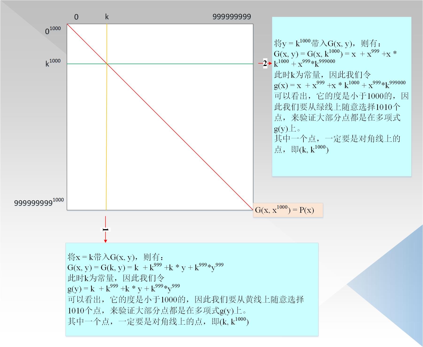
The verifier calculated all the points (yes, 10 ^ 18 points in total, scared BB), and formed a Merkel tree. The verifier randomly selects a row and a column, as shown by the red line 1/2 in the figure. For each column, it is generated by a polynomial with a degree of less than 1000. For each row, it is a polynomial with a degree of x less than 1000. generate. The verifier randomly selects 1010 points from the rows / columns to verify whether the points on the corresponding row / column are on a polynomial with a degree of less than 1000. It should be noted that because the points of P (x) are all in the pairs in the figure above Diagonal, so we have to make sure that the points on the diagonal corresponding to each row / column are also on the corresponding polynomials with degree less than 1000, that is, 1010 points must include diagonal points.

Reliability analysis: If the degree of the original polynomial is actually less than 10 ^ 6 +10999, that is, P (x) = x + x ^ 999 + x ^ 1001 + x ^ 1010999, then the corresponding G (x, y) is G (x, y) = x + x ^ 999 + x * y + x ^ 999 * y ^ 1010, that is, for each x, G (x, y) is a univariate polynomial function about y, and the degree d <1010 , So all points in each column in the figure below are on polynomials with degree d <1010, not on polynomials with d <1000. So if the prover still claims the degree d <1000,000 of the polynomial P (x), the verification will fail. The same is true in other scenarios.

Is it possible that the malicious prover still generates evidence in the form of G (x, y) = x + x ^ 999 + x * y + x ^ 999 * y ^ 999? Will this pass?

We know that during the verification, we emphasized that the point on the diagonal must be on the polynomial. We know that the polynomial form corresponding to the diagonal at this time is

P (x) = x + x ^ 999 + x1001 + x ^ 999999, and the actual P (x), which we label here as P` (x), has the form:

P` (x) = x + x ^ 999 + x ^ 1001 + x ^ 1010999

Therefore, if the verifier chooses exactly the intersection of two polynomials, the verification will pass. In fact, the two polynomials have at most about 1,000,000 intersections. However, since the randomly selected points are not selected by the prover, they are determined by The root of the Merkel tree is randomly generated by the seed, so the prover has no chance to do evil, and can choose those points that can pass the verification.

Since there are 10 ^ 9 points in total, a random point is selected, and the probability of successful verification is 10 ^ 6/10 ^ 9 = 10 ^ (-3). If k rows are selected, the probability of success is only 10 ^ ( -3k).

It can be seen from the above that the verifier and the prover only need to interact with 1010 * 2 * k points to complete the verification. If k = 10, then 1010 * 2 * 10 = 20100 << 10 ^ 6.

1. Although the above implementation completes LDT verification when the number of interactions is less than D, the complexity of the prover is too large, and the complexity of at least 10 ^ 18 is much larger than the original calculation, so some optimization schemes are needed to reduce the complexity. Not much to say, direct introduction of finite fields, after all, in actual projects, we do not want the value itself to be too large. The conclusion of Fermat's little theorem is directly quoted: in a finite field p, if (p-1) can be divisible by k, then there are only (p -1) / k + 1 images mapping x => x ^ k. Figure 5 below uses p = 17 and the mapping x => x ^ 2 as an example:

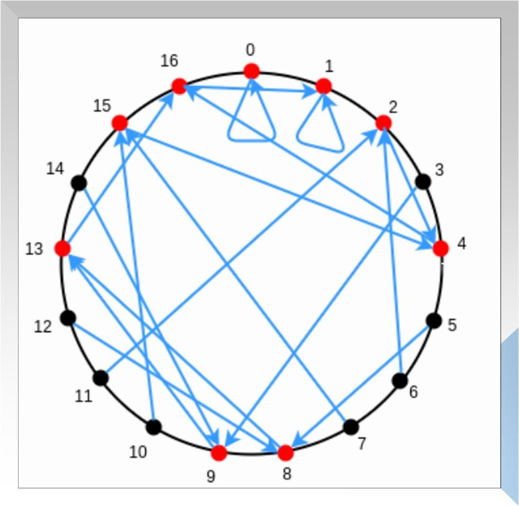
In the figure, red is the image of x ^ 2 in the finite field p, which consists of (p-1) / 2 + 1 = 9 in total. At the same time, we can find that the images of 9 ^ 2 and 8 ^ 2 are the same, the images of 10 ^ 2 and 7 ^ 2 are the same, and so on, the images of 16 ^ 2 and 1 ^ 2 are the same. Remember this phenomenon, and Zhang Tu's understanding is helpful.

Therefore, in this example, we choose a prime number p = 1000,005,001, which satisfies:

• Prime
• p-1 is divisible by 1000
• p must be greater than 10 ^ 9

Therefore, in the finite field p, the image of x => x ^ 1000 has (p -1) / 1000 = 1000,005 in p, so Figure 4 can be transformed into the form of Figure 6:

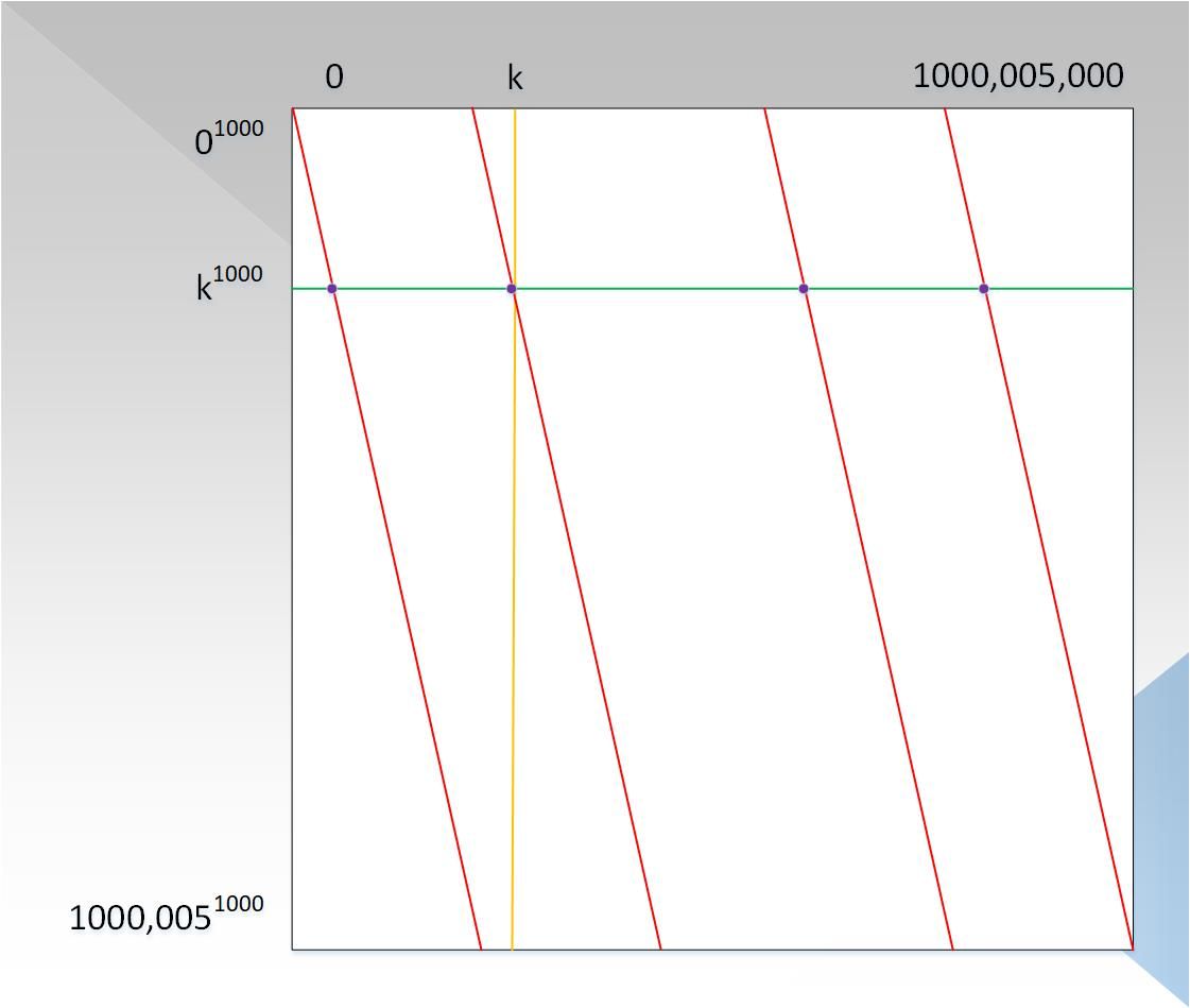
It can be seen that the column coordinates have become 10 ^ 6 elements, and the diagonal lines have become parallel lines, with a total of 1,000. Remember the special phenomenon of Fermat's Little Theorem above? This is the reason for the distribution of diagonals. The reader tries to understand (maybe the reader will think that the diagonals should be zigzag, not this parallel form. Maybe you are right, but this does not affect the verification process. ). At this time, the complexity of the prover has been reduced from 10 ^ 18 to 10 ^ 15, and the proof and verification process is still the same as described in step 3.

1. Can we continue to optimize it? The answer is yes. Recalling the verification process described above, for each row / column, the verifier must obtain 1000 points to interpolate and degenerate a polynomial with a degree less than 1000. Look closely at Figure 6. For each row, there is not 1000 in the original data. Number? Then we simply select these points to interpolate a polynomial with a degree of less than 1000, and then just randomly ask the prover to calculate any column, and prove that the points along the column are on the polynomial with degree less than 1000, and the points on the column are also On the corresponding row polynomial using the original data interpolation. At this point, the prover complexity was reduced from 10 ^ 15 to the power of 10 ^ 9.
2. Summary: Personal understanding, from step 1 to step 5, is actually the selection process from PCP to IOP.
   1. The PCP requires the prover to generate all the evidence, and then the verifier randomly selects a part of it for verification several times, but the complexity of the prover is still high;
   2. IOP requires the prover not to generate all the evidence. According to multiple interactions, only a part of the evidence needs to be generated each time, so that the complexity of the proof and D are approximately linear.
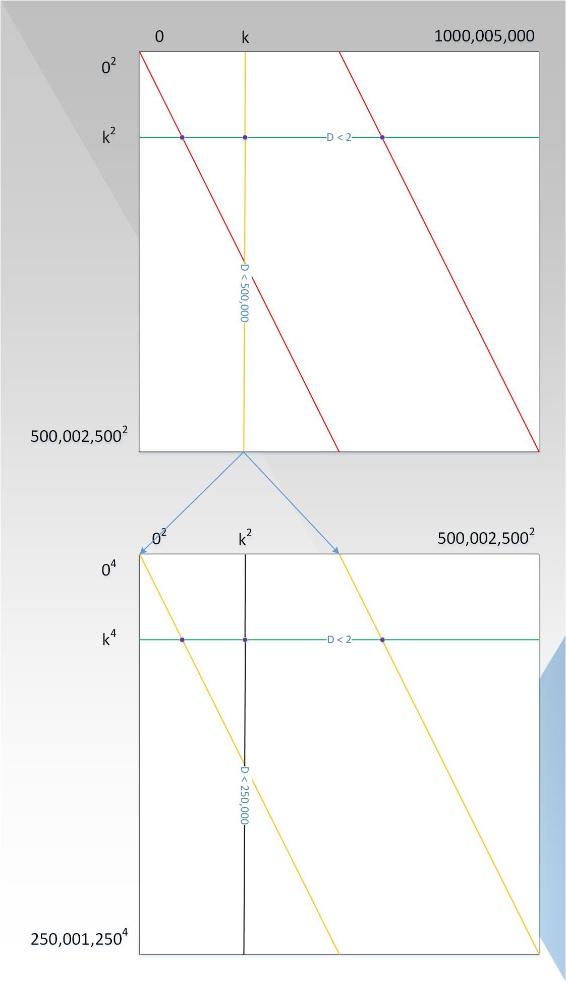
3. The prover's complexity has been reduced to a quasi-linear relationship with D. Although the verifier's complexity is sub-linear and the number of interactions is already lower than D, can it be optimized to a lower level? Based on the optimal setting of proof complexity, we continue to explore the optimization path of verification complexity, reviewing P (x) = x + x ^ 999 + x ^ 1001 + x ^ 999999 = x + x * (x ^ 2) ^ 499 + x * (x ^ 2) ^ 500 + x * (x ^ 2) * 499999, let G (x, y) = x + x * y ^ 499 + x * y ^ 500 + x * y ^ 499999, Then when y = x ^ 2, there is G (x, y) = G (x, x ^ 2) = x + x * (x ^ 2) ^ 499 + x * (x ^ 2) ^ 500 + x * (x ^ 2) * 499999 = P (x). The final diagram should look like Figure 7 below:

We can see from the figure:

• Proof, the complexity is still 10 ^ 9 power;
• The points on each line are on polynomials of degree d <2 because when y takes a fixed value, G (x, y) is a polynomial of degree about x;
• The points on each column are on polynomials with degree d <D / 2. The prover needs to prove that the polynomial is less than D / 2. Assume that the polynomial is P1 (x). At this time, it is not the verifier that chooses greater than D / 2. Point to verify, because the verification complexity is still not low enough, but this column uses a process similar to P (x) again, as shown in the lower figure in Figure 7, and this cycle, until you can directly judge The degree of the polynomial on the column is similar to the row.

to sum up

At this point, this article is over. To summarize, this article mainly explains the following:

• How to convert problem forms-Arithmetization
• Why LDT is needed-for verification simplicity
• The approximate process of LDT-dichotomy verification, similar to FFT
• Reduce the complexity of LDT-finite field + IOP

As for the detailed process of LDT, it will be left to the last article in this series, so stay tuned.

Thank you all, welcome criticism and correction, if you have any questions or questions, you can leave a message.

We will continue to update Blocking; if you have any questions or suggestions, please contact us!