The Impact of Cryptocurrency Wealth on Family Consumption and Investment

Cryptocurrency Wealth's Impact on Family Consumption and Investment

Author | Darren Aiello, Scott R. Baker, Tetyana Balyuk, Marco Di Maggio, Mark J. Johnson, Jason D. Kotter

Source | NBER

Translation | Xu Hecong

Recently, NBER published a working paper titled “The Effects of Cryptocurrency Wealth on Household Consumption and Investment”. The paper uses transaction-level data from millions of accounts to identify cryptocurrency investors and assess the impact of individual cryptocurrency wealth fluctuations on household consumption, stock investment, and the local real estate market. The paper estimates that the marginal propensity to consume (MPC) of unrealized cryptocurrency returns is more than twice as large as the MPC of unrealized equity returns, but smaller than the MPC from exogenous cash flow shocks. This MPC is mainly driven by increases in cash expenditures and mortgage loans. In addition, households sell cryptocurrencies for both discretionary spending and housing expenses. Therefore, cryptocurrency wealth leads to an increase in housing prices, and counties with higher cryptocurrency wealth experience faster growth in housing values after high cryptocurrency returns. The results indicate that cryptocurrencies have important spillover effects on the real economy through consumption and investment in other asset classes. The core part of this article has been translated by the Institute of Fintech Research at Renmin University of China.

• When the post-2000 generation who entered the circle in 2020 are called OG, reviewing the three cycles of the crypto industry in the past ten years.
• Bold Bitcoin Strategy by BlackRock Suggesting High Bitcoin Portfolio Allocation
• Huobi Research Institute’s latest research report | A comprehensive analysis of the current situation, risks, and future development of the cryptocurrency financial product market.

Introduction

Over the past decade, cryptocurrencies have gone from relatively unknown to reaching a peak global market value of over $3 trillion. More and more American households are including cryptocurrencies as part of their investment portfolios, and the extreme volatility of cryptocurrencies has allowed many investors to quickly accumulate wealth. While the cryptocurrency market has experienced rapid growth, there is uncertainty about its spillover effects on the broader economy, which may have implications for policymakers and household welfare. Although some attention has been focused on cryptocurrencies and financial stability, the limited availability of data due to the anonymity of blockchain transactions has restricted research on the impact of cryptocurrency introduction on individual household investment and consumption behavior, as well as its spillover effects on other asset classes.

This paper uses transaction-level data from millions of US households’ bank accounts and credit card payments to analyze how cryptocurrency wealth affects the broader economy. Specifically, this paper tracks how household consumption responds to changes in cryptocurrency wealth and evaluates the causal effect of this wealth on local real estate market prices. The paper identifies cryptocurrency users based on the timing of funds flowing in and out of major cryptocurrency exchanges and infers their cryptocurrency wealth. While most cryptocurrency users have relatively small investments in this asset class, many hold amounts equivalent to several months’ worth of consumption in these accounts. The paper first describes the characteristics of cryptocurrency users by combining a large sample representing American households with complete financial transaction records. This allows the paper to compare the income and consumption patterns of cryptocurrency users and non-cryptocurrency users.

The focus of this article is the impact of cryptocurrency returns on consumption and investment decisions. The article found that people who adopt cryptocurrencies have higher incomes, which is consistent with some survey data, and are more likely to deposit funds into traditional brokerages. Consistent with these income differences, people who adopt cryptocurrencies spend a higher proportion of their income on categories such as entertainment and dining. On average, households seem to view cryptocurrencies as part of a larger investment portfolio. Cryptocurrency users tend to actively trade in the stock market, often investing in both cryptocurrency assets and traditional stock securities. Some evidence suggests that after obtaining significant returns, households rebalance their investment portfolios by selling cryptocurrencies and depositing funds into traditional brokerages. Despite signs of financial maturity, this article also found that some cryptocurrency users are driven by the returns of cryptocurrencies, and overall adoption seems to be significantly influenced by high returns. The time with the highest monthly increase in cryptocurrency users in the sample of this article was in 2017, when Bitcoin experienced its highest return in history.

Next, this article examines the impact of household-level cryptocurrency returns on consumption. The article uses monthly panel data for a user and observes changes in consumption patterns following changes in cryptocurrency wealth. On average, this article estimates the marginal propensity to consume (MPC) of cryptocurrency wealth to be $0.08. Qualitatively, this is similar to the consumption response to real estate and securities appreciation, but quantitatively it is 2 to 3 times larger. At the same time, the MPC is approximately one-third of the MPC for one-time income shocks. This suggests that households view cryptocurrency returns as a mix of external cash flow shocks and traditional investment portfolios. Although cryptocurrency returns during this period were similar to lottery returns, the estimated MPC is much smaller, with MPC ranges in lottery-winning studies ranging from 50% to nearly 100%. Overall, the increase in household cryptocurrency wealth in the sample of this article has a total impact on consumption of approximately $20 billion. If non-retail cryptocurrency income consumption is similar to the estimates in this article, the total effect in the United States could be between $80 billion and $100 billion.

In the short term, cryptocurrency wealth has a larger impact on high-income households, and the most significant identifiable consumption changes come from higher mortgage expenses. Housing consumption changes at the individual level suggest that cryptocurrency returns may have spillover effects on the local economy-increased demand for housing may put pressure on local house prices. However, two challenges make it difficult to estimate the impact of cryptocurrency wealth on house prices. Simple regression estimates may face reverse causality issues, as higher house prices may lead households to withdraw from cryptocurrency investments to purchase homes. In addition, counties that become wealthier may simultaneously increase investments in all assets, which may be due to changes in education, occupation, or industry concentration. In the final section of the paper, this article addresses these issues by using two independent natural experiments to estimate the causal impact of county-level cryptocurrency wealth on local house price growth.

The first experiment takes advantage of the maximum increase in Bitcoin price during the sample period (end of 2017) and considers the impact of cryptocurrency wealth as a county-level phenomenon. Before the price increase, counties with higher per capita cryptocurrency wealth experienced cryptocurrency returns of around 1400%. To mitigate some concerns about reverse causality, this study uses a difference-in-differences approach and fixes cryptocurrency wealth during the pre-period, noting the absence of differential trends before the price surge. This study further demonstrates that counties with higher cryptocurrency wealth experienced a significant increase in cryptocurrency withdrawals after the Bitcoin price shock, but traditional brokerage withdrawals did not experience discontinuous changes. The study finds that in the months following the price increase, counties with higher cryptocurrency wealth in the pre-2017 period experienced significantly higher housing price growth. Compared to counties with lower cryptocurrency wealth, counties with higher cryptocurrency wealth saw housing price growth approximately 46 basis points faster, explaining around 12% of the standard deviation in housing price growth during this period.

This study extends the basic concept of difference-in-differences estimation to the entire time series using two-stage least squares (2SLS). The study uses the passive returns of county-level cryptocurrency wealth, defined as the county-level cryptocurrency wealth value based on the 12-month prior returns of Bitcoin and Ethereum, as an instrument for county-level cryptocurrency wealth growth. Using passive cryptocurrency portfolio returns as instruments for county-level cryptocurrency wealth changes, the study finds that an increase in cryptocurrency wealth leads to a significant increase in housing prices. It is estimated that an increase in per capita county-level retail cryptocurrency wealth over the next 6 months would result in an increase of approximately $0.21 in county-level housing prices.

Because this instrument is based on historical cryptocurrency portfolios, it alleviates concerns about reverse causality. However, to establish the impact of cryptocurrency wealth on local housing prices, this instrument must satisfy the exclusion restriction, meaning that the passive gains from cryptocurrency wealth are unrelated to any other non-cryptocurrency wealth changes that may affect housing prices. The quasi-randomness of cryptocurrency returns makes it unlikely that most sources of wealth correlated with cryptocurrency returns and historical county-level cryptocurrency wealth are simultaneously related. The most likely exception is stock market returns. Counties with higher cryptocurrency wealth also tend to participate in the stock market, and cryptocurrency returns are positively correlated with stock market returns, at least during certain periods. However, the 2SLS results of this study are robust to modifying the instrument to use cryptocurrency returns that exceed market stock returns.

Unlike papers that describe the characteristics of cryptocurrency investors or cryptocurrency trading behavior, this study investigates the interaction between cryptocurrency price volatility and household consumption and investment behavior. Compared to previous papers, the data used in this study allows for the linkage of a broader set of U.S. retail cryptocurrency traders with relatively complete records of other financial transactions. This study examines household consumption decisions after realizing cryptocurrency returns, a new asset class with extreme volatility. Comparing these consumption decisions with decisions made after stock or housing returns can reveal how households treat cryptocurrency compared to other asset classes. Additionally, this study utilizes regional wealth shocks to test for spatial variation in economic impacts.

The rest of this article is as follows. Section 2 introduces the transaction-level dataset of this article. Section 3 discusses the role of cryptocurrencies in household investment decisions. Section 4 examines the consumption response to cryptocurrency wealth at the household level. Section 5 introduces the causal effect estimation of county-level cryptocurrency wealth on local housing prices. Section 6 concludes.

Data

2.1 Transaction Data

The data provider of this article is a large financial analytics company specializing in extracting and analyzing data from anonymous bank, credit card, and debit card transactions of millions of households in the United States. The provider primarily contracts with financial institutions and fintech companies to provide data and personal financial management services to their clients and is able to aggregate financial information from users’ financial accounts. Therefore, under the condition of conducting banking business with specific financial institutions, there are no additional user choices in the database, and user churn is minimal.

The data in this article is limited to bank, credit card, and debit card transactions and does not include transactions conducted in other types of accounts (such as brokerage accounts), but deposits and withdrawals from these accounts are usually observable. Each transaction contains a lot of information. For example, this article is able to observe the exact date and amount of a transaction, as well as whether the transaction was conducted in person or remotely. Using the textual description information attached to the transaction, the transactions are classified into 43 different categories (such as salary, ATM withdrawal, groceries, mortgage payments, medical expenses). For most transactions, the merchant name and the actual location at the city or zip code level are also observable.

The complete database covers 60 million U.S. users and billions of transactions from June 2010 to September 2022. The database experienced a large-scale expansion of users in the early years, so this article focuses on data from 2014 onwards to mitigate concerns about population changes. Although this data allows this article to see a wealth of details about users’ financial transactions, demographic statistics such as age, gender, or race are not observable. However, the data provider provides a monthly panel to estimate users’ current place of residence (city). For many users, this article is also able to infer their postal codes of residence based on the actual locations of merchants that frequently appear in their transactions.

2.1.1 Validation of Consumer Transaction Data

Although the data of this article is not randomly sampled from the population, overall, it seems to be highly representative of the entire economy. Many other transaction databases are sampled from highly selective populations (e.g., those interested in using fintech applications for lending or debt repayment assistance). In contrast, the data provider of this article collaborates with large financial institutions that cover a significant portion of the U.S. population, reducing concerns about highly selective samples.

To validate the broad representativeness of the data, this article compares the consumer data observed in this article with merchant data obtained from the Census Bureau’s retail sales surveys. These surveys are used by the U.S. Census Bureau to estimate monthly retail sales by merchant category. Figure 1 summarizes the monthly observable transactions in a range of categories (automotive and fuel, general merchandise, groceries, personal/household, medical, and food services) from the data of this article.

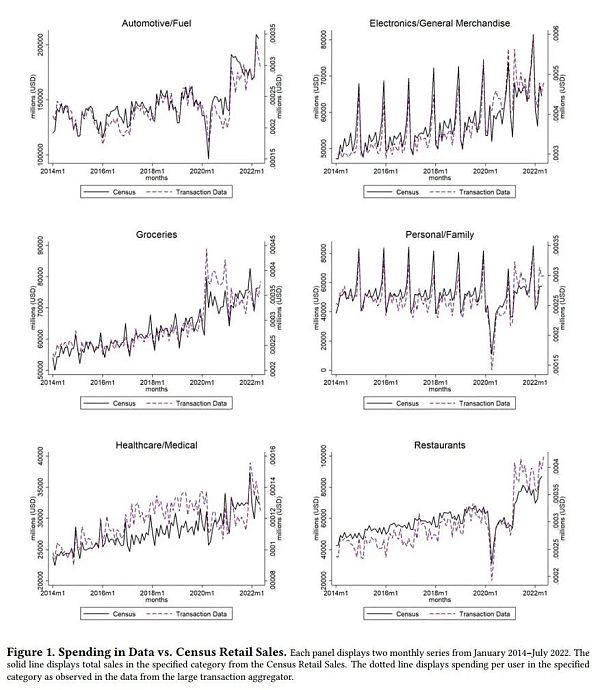
Figure 1 Expenditure vs Total Sales

This figure shows that the consumption trends from 2014 to 2022 are very similar in the data of this article and the Census Bureau’s retail sales survey. On average, the correlation between monthly consumption from these two sources is about 0.90. The series with the lowest correlation is the medical and healthcare category, which is also expected in this article to have a large proportion of household pre-tax or third-party expenditures, leading to differences between household observable consumption and reported income by retailers. The data also seems to be representative across counties. In Appendix Figure A.1, this article plots a grouped scatter plot of county weights calculated by population and user weights in the transaction data of this article.

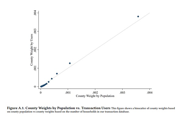
Figure A.1 County Weights by Population vs Transaction Users

Another common issue when using transaction data is whether this article can observe the overall situation of income and consumption transactions related to a given user. For this data source, if a household only holds and uses credit cards from financial institutions that have signed contracts with the aggregate service, this article will observe the complete transactions of that household. Although it is unlikely that the users in the data are completely like this, this article focuses on a high-quality subset of users that are more likely to exhibit this behavior at the household level. The data provider ranks the quality of transaction data based on completeness and account tenure. This article focuses on a high-quality subset of users randomly sampled from the top 10% of this quality indicator, totaling 95,965 users.

2.2 Identifying Cryptocurrency Exchange Transactions

Using the text descriptions and merchant information attached to each transaction in this article’s database, this article is able to identify transactions that represent deposits or withdrawals to and from popular cryptocurrency exchanges. This article lists major cryptocurrency exchanges and conducts extensive manual checks to identify various text string variants representing transactions with major exchanges (e.g., “Coinbase.com debit card purchase” or “GeminiTrustCo transfer”). These exchanges include Coinbase, Binance, Gemini, Crypto.com, Kucoin, Cryptohub, Blocket, CEX.io, and Bitstamp. The focus of this article is on cryptocurrency exchanges, which means the estimate of retail cryptocurrency wealth in this article is necessarily underestimated, as some investors hold cryptocurrencies in private wallets obtained through direct purchases or mining, and it is difficult to determine how much retail cryptocurrency is held outside of exchanges. Since 2015, about 75% of Bitcoin transactions have occurred between exchanges. This suggests that this article may capture most of the deposits and withdrawals from retail cryptocurrency exchanges.

Although users can interact with exchanges using bank transfers, debit cards, and credit cards, the majority of transactions are conducted through checking accounts or debit cards, with credit cards accounting for less than 2% of cryptocurrency transactions. Furthermore, while this article observes deposits and withdrawals, nearly 90% of transactions with these exchanges are deposits, reflecting the significant growth in deposits to these exchanges as cryptocurrency investment becomes more popular nationwide. Approximately 90% of the deposit and withdrawal amount occurs on Coinbase. Gemini accounts for an additional 5% of the amount, while the other 9 exchanges account for less than 5% of the total amount.

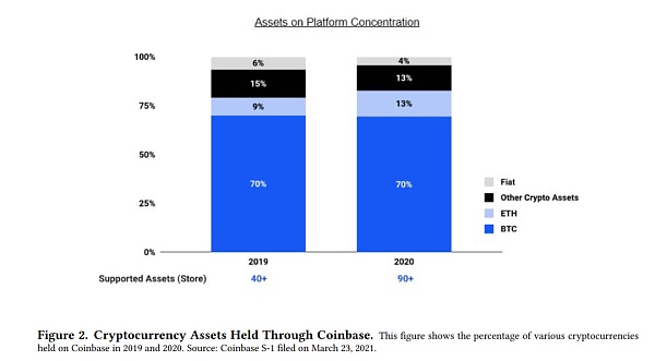
Figure 2: Cryptocurrency assets held by Coinbase

This article did not observe the actual cryptocurrency purchased by households. However, since the majority of cryptocurrency transactions in this article occurred on the Coinbase exchange, it is possible to understand potential purchasing behavior by examining the overall asset holdings on Coinbase. Figure 2 shows the asset portfolio on Coinbase in 2019 and 2020. The majority (about 70%) of assets held on Coinbase are Bitcoin; approximately another 10% of assets are Ether. Importantly, there is almost no cash (i.e. fiat currency) held on Coinbase. Based on this data, deposits to (withdrawals from) Coinbase most likely represent purchases (sales) of Bitcoin or Ether. Therefore, this article estimates the total cryptocurrency portfolio value of households as

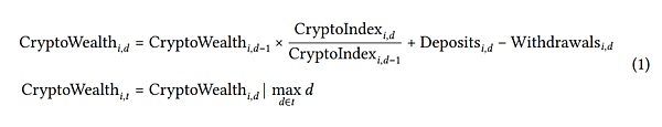
where the cryptocurrency wealth of household i on day d is equal to the wealth of the household on the previous day multiplied by the daily return of the specific cryptocurrency index (CryptoIndex?,d) for the household. This index consists of Bitcoin and Ether, weighted according to the household’s asset portfolio weights on the previous day. Then this article adds the net deposits to the cryptocurrency exchange on the day. This calculation assumes that all funds deposited into the cryptocurrency exchange are used to purchase a basket of Bitcoin and Ether on the day of the transaction, with the weights allocated based on the relative total market value of these currencies on that day. This article assumes that funds withdrawn from the cryptocurrency exchange are distributed proportionally to Bitcoin and Ether according to the asset portfolio weights on the previous day. This article further assumes an initial cryptocurrency wealth of zero and then calculates the monthly cryptocurrency wealth (CryptoWealth?,t), which is the investment portfolio value of the household on the last day of month t.

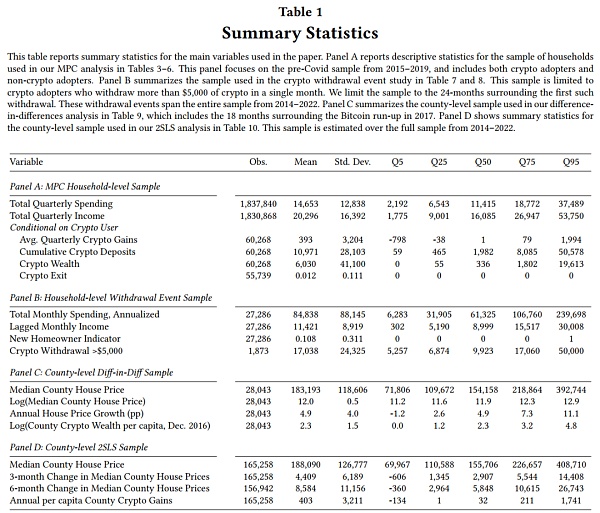
Table 1 reports summary statistics of household cryptocurrency wealth. On average, the cryptocurrency investment portfolio value of cryptocurrency users in this article is approximately $6,000. However, due to a few users having very large portfolios, this average is skewed. The median of the cryptocurrency investment portfolio is only $336, and the 75th percentile is $1,800. In comparison, by 2022, the largest portfolio value is approximately $9 million.

Table 1 Descriptive statistics

The skewness of cryptocurrency investment portfolio wealth roughly matches the skewness of equity holdings by U.S. households. In Appendix Figure A.5, this article compares the distribution of cryptocurrency wealth in the sample with household equity holdings based on the Federal Reserve’s Survey of Consumer Finances (SCF). This article observes very similar patterns between cryptocurrency and equity holdings – only a small portion of wealth is held by households below the 80th percentile, and the majority of equity wealth is evenly distributed between the 80th-99th percentiles and the highest percentile. This analysis suggests that any differences observed between cryptocurrency wealth and equity wealth consumption in this article are unlikely to be driven by differences in the distribution of these two types of wealth.

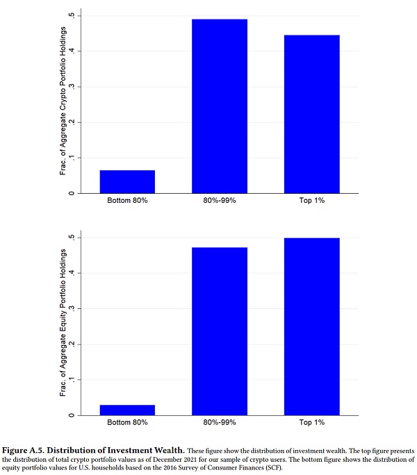
Figure A.5 Wealth Distribution of Investments

In the account-level sample of this article, about 16% of households made deposits to retail cryptocurrency exchanges at some point between 2014 and 2022. According to recent survey data, this proportion is very close to the estimated proportion of the U.S. population that has traded cryptocurrencies.

2.3 Other Data

Transaction data providers use algorithms to determine the city and state where households are located. This article uses ArcGIS to geocode the counties associated with the city. In the analysis in Section 5, this article aggregates the value of cryptocurrency portfolios at the county-month level. In this analysis, a larger sample of about 6 million households is used to obtain a more accurate measure of county-level cryptocurrency wealth. This data is merged with the monthly county-level Zillow Home Value Index (ZHVI). ZHVI is a smoothed, seasonally adjusted house price index that reflects typical home prices at the county-month level.

2.4 Composition of Cryptocurrency Investors

Cryptocurrency is a rapidly growing asset class with a global market value exceeding $1 trillion. Despite its rapid growth, the decentralization and anonymity of blockchain transactions make it difficult for this article to understand who is investing in cryptocurrencies and the motivations behind these investment decisions. This article expands on this research by providing evidence on the investment behavior of a large representative sample of U.S. households based on actual cryptocurrency transaction data. As this article observes not only cryptocurrency transactions but also complete payment transactions, it becomes the first to describe the consumption patterns of cryptocurrency investors in comparison to other households.

This article focuses on several key features of the retail cryptocurrency market development that are relevant to later analysis. Figure 3 shows the development of deposits and withdrawals from cryptocurrency exchanges. This article examines the correlation between the sum of cryptocurrency deposits and withdrawals and cryptocurrency returns (defined by market-cap weighted indices of Bitcoin and Ethereum) in a 10% sample of the 60 million households covered in this article’s transaction data. The four panels in the figure display cryptocurrency deposits, withdrawals, new users, and net deposits. The substantial cryptocurrency returns are evident. After significant increases in cryptocurrency prices, there are surges in the number of new users and total cryptocurrency deposits. In fact, the largest surge in new users in this article’s sample occurred at the end of 2017 when cryptocurrency returns reached their highest 12-month return. Interestingly, withdrawals also surged during this period, indicating that at least some households cashed out their cryptocurrency earnings.

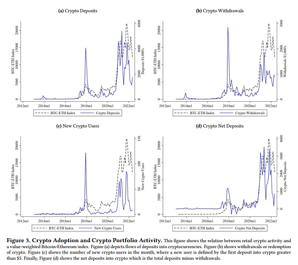
Figure 3 Adoption of Cryptocurrency and Cryptocurrency Portfolio Activity

One advantage of this article’s transaction data is that it allows for the observation of consumption patterns of households that invest in cryptocurrencies as well as households that do not invest in cryptocurrencies. Table 2 presents the average monthly income, expenses, and the proportion of different categories of expenses for households that invest in cryptocurrencies and households that do not invest in cryptocurrencies. Some key patterns emerge from the data. People who invest in cryptocurrencies have higher incomes: the average monthly income of those who invest in cryptocurrencies is $8,176, compared to $7,356 for those who do not invest. Perhaps not surprisingly, given the income difference, people who invest in cryptocurrencies also engage in more active investing in traditional brokerage accounts.

Table 2 Descriptive Statistics of Samples and Cryptocurrency Investors

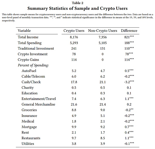
Despite income differences, the overall expenditure patterns of households investing in cryptocurrencies and those not investing in cryptocurrencies are relatively similar. The biggest difference lies in discretionary spending. Consistent with higher disposable income, individuals investing in cryptocurrencies have a budget expenditure in entertainment/travel that is about 1.1 percentage points higher than those not investing in cryptocurrencies, and about 1.2 percentage points higher in restaurants. Individuals investing in cryptocurrencies also have higher expenditure on cash/check purchases.

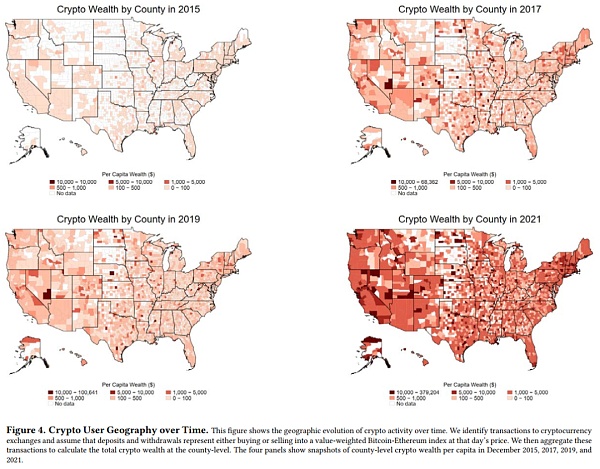
Figure 4 Geographical Distribution of Cryptocurrency Wealth over Time

Figure 4 shows the geographical distribution of cryptocurrency wealth over time. This study aggregates the total cryptocurrency wealth value at the county level and divides it by the number of households in that county. Then, this study presents county maps for the end of 2015, 2017, 2019, and 2021. In 2015, most coastal counties had small wealth, less than $100 per household, and the inland areas of the continental United States had little cryptocurrency participation. In 2017, during the first rise in cryptocurrency prices, dozens of counties across the United States began accumulating cryptocurrency wealth of $1,000 or more per household. However, by the end of 2021, the cryptocurrency wealth per household in most populated U.S. counties had reached at least $1,000, and in some counties, it had reached tens of thousands of dollars. Counties with the highest per capita cryptocurrency value are concentrated in California, Nevada, and Utah. This geographical variation suggests that cryptocurrency wealth may have different impacts on local economies in different counties, which will be explored in section 5.

Investment After Cryptocurrency Wealth Growth

Table 2 results show that cryptocurrency users are more likely to have traditional brokerage investments compared to those who do not invest in cryptocurrencies. To some extent, if cryptocurrency investors have a certain level of financial knowledge, it is expected that they will rebalance a significant portion of their cryptocurrency earnings into traditional investments. However, survey data suggests that household cryptocurrency investors may view cryptocurrencies as substitutes for traditional investments. For example, a survey by the Pew Research Center in 2022 found that among respondents who claimed to have invested in cryptocurrencies, 78% said that one of their motivations was to have a different investment method, 54% believed that investing in cryptocurrencies is easier than traditional investments, and 39% said that they have more confidence in cryptocurrencies than other investments. If these expressed views in the survey are representative, cryptocurrency users are likely to increase their cryptocurrency investments rather than rebalancing cryptocurrency earnings into the stock market.

This study evaluates the relationship between cryptocurrency earnings and future investments to explore the extent to which cryptocurrency users rebalance their cryptocurrency investment portfolio. In Figure 5, this study plots a cross-sectional scatter plot of total brokerage deposits and total cryptocurrency deposits, with cryptocurrency deposits not exceeding $100,000. There is a strong positive correlation between the two types of deposits. However, for most households, the total amount of brokerage deposits far exceeds the total amount of cryptocurrency deposits. This relationship becomes relatively stable when it comes to high-end cryptocurrency deposits. For example, for the average user depositing $20,000, the amount invested in traditional brokerage accounts is 2-3 times that of the cryptocurrency deposit, while for the average user depositing $50,000, the amount deposited in brokerage accounts is roughly equal. This suggests that there are two types of retail cryptocurrency investors. For one type of investor, cryptocurrencies only represent a small portion of their investment portfolio, while traditional brokerage deposits dominate. On the other hand, there is also a small group of cryptocurrency investors who invest relatively little in traditional brokerage institutions but have a significant investment in cryptocurrencies.

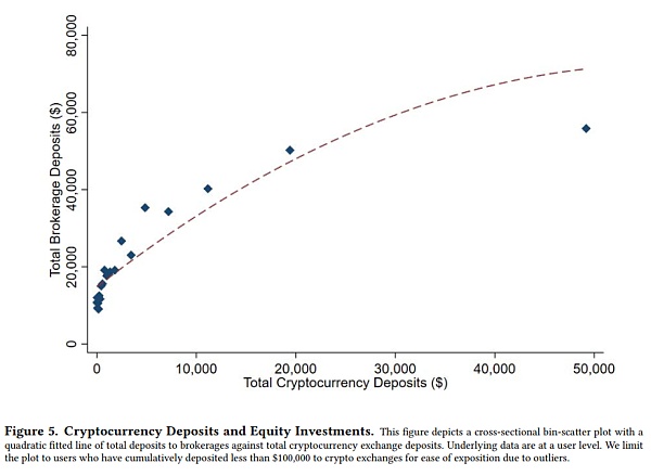
Figure 5 Cryptocurrency Deposits and Equity Investments

To further explore this relationship, this paper studies household investment decisions after cryptocurrency returns (and losses). For each household, this paper defines the average quarterly cryptocurrency returns as

Where the calculation of CryptoWealth is shown in equation 1, and NetWithdraw?,q−3→q is defined as the total cryptocurrency withdrawals minus total cryptocurrency deposits for household i in the past four quarters (including the current quarter q). Therefore, CryptoGains include both realized and unrealized gains experienced by households.

Table 1 reports the distribution of average quarterly cryptocurrency returns. Among cryptocurrency investors, the average quarterly cryptocurrency wealth growth is about $390, with a standard deviation of $3200. About 43% of households experienced losses in the quarter. In cases of positive returns, the average quarterly cryptocurrency wealth growth is about $1060. In cases of losses, the average quarterly loss is about $433.

This paper estimates the relationship between cryptocurrency returns and future investment decisions through the following form of OLS regression:

The dependent variable Invest?,q represents the total funds invested by household ? in quarter q. This paper examines both cryptocurrency investments and traditional brokerage investments. The paper includes household (??) and quarter-state (??,?) fixed effects, and controls for lagged income and previous investment deposits. The regression includes both cryptocurrency users and non-cryptocurrency users; although non-cryptocurrency users do not have cryptocurrency returns, they serve as an important control group, helping to estimate investment behavior trends. This paper truncates cryptocurrency returns at the 1st and 99th percentiles to mitigate concerns about measurement errors in cryptocurrency wealth, and trims income at the 1st and 99th percentiles to exclude households with unreliable trading data. This paper clusters standard errors at the household level. The estimated value of interest ? represents the additional dollars invested in cryptocurrency exchanges or traditional brokerage firms in a quarter, equivalent to the average quarterly cryptocurrency returns per dollar obtained last year.

Table 3 reports the estimates of equation 3. In column 1, this paper estimates the relationship between cryptocurrency returns and future cryptocurrency deposits. This paper finds that the greater the growth of cryptocurrency wealth, the more funds are deposited in cryptocurrency exchanges—an increase of $1 in cryptocurrency wealth means an additional $0.06 of cryptocurrency deposited per quarter. This result suggests that there is a small but significant momentum effect in retail cryptocurrency investments.

Table 3: Cryptocurrency Returns and Investments

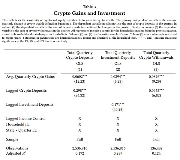
In column 2 of Table 3, this study examines the relationship between cryptocurrency wealth growth and future stock investments, using traditional brokerage deposits as a proxy. The study finds that the greater the wealth growth in cryptocurrency, the more traditional investments are made. An increase of $1 in cryptocurrency wealth is correlated with an increase of $0.03 in traditional investments. This result suggests that some households may reallocate their cryptocurrency returns into traditional investments.

To better understand the possibility of portfolio rebalancing, this study estimates the relationship between cryptocurrency returns and future cryptocurrency withdrawals in column 3. The study finds a positive and significant relationship between cryptocurrency returns and future cryptocurrency withdrawals; an increase of $1 in cryptocurrency wealth implies an increase of $0.09 in future cryptocurrency withdrawals. Importantly, the estimates in columns 1 and 2 come from different households, indicating that some households exhibit momentum in cryptocurrency investments, thus amplifying unrealized cryptocurrency returns, while others extract cryptocurrency returns and rebalance their portfolios.

Consuming from Cryptocurrency Wealth

How does the increase in cryptocurrency wealth affect household consumption? This study re-estimates Equation 3 with total quarterly household consumption as the dependent variable to answer this question. The β in these regressions can be interpreted as the marginal propensity to consume (MPC) of each additional dollar of new cryptocurrency wealth. The results are reported in Table 4. In the full sample, the study finds a small, statistically insignificant MPC.

Table 4: Cryptocurrency Returns and Total Expenditure

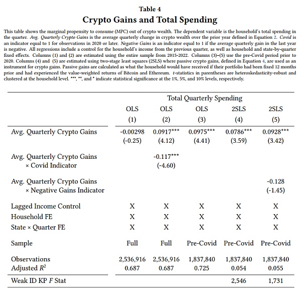
The MPC estimates suffer from a potential confounding factor, as the last two and a half years in the study sample occurred after the Covid pandemic. Overall expenditure declined during this period, consistent with limited travel and other discretionary spending opportunities. The decline in expenditure was particularly pronounced for high-income households, which are also more likely to be involved in cryptocurrency investments. These data characteristics are likely to bias the MPC estimates of cryptocurrency wealth during Covid to be lower. To address this issue, in column 2, the study interacts cryptocurrency returns with quarterly indicators of the Covid period. The study finds a strong negative correlation between cryptocurrency returns and expenditure during Covid; however, before Covid, the MPC of cryptocurrency wealth was approximately $0.09 for each additional dollar of cryptocurrency returns. In column 3, the study restricts the sample to the period before Covid and obtains a similar MPC. This MPC of cryptocurrency wealth is approximately three times the estimated MPC of equity wealth, which is approximately $0.03 for individuals with similar wealth distribution points. However, it is lower than the estimated MPC of lottery winnings, which is approximately $0.50. Therefore, households treat cryptocurrency returns more like lottery winnings than equity returns, but it is more similar to equity returns than actual lottery winnings.

One issue with MPC is that the realized encrypted returns may be endogenously related to household expenditures. If investors anticipate large expenses, they may choose to cash out part of their investment portfolio in advance, especially if they believe that cryptocurrency prices may fall. Alternatively, investors may double down on their investments in cryptocurrencies, hoping that high returns will generate the necessary wealth to cover their expenses. If investors’ beliefs about cryptocurrency returns are correct, these types of behaviors will lead to an upward bias in the ordinary least squares estimates in this paper, as observed expenditures will increase precisely when realized plus unrealized encrypted returns are larger.

To address these issues, this paper constructs a tool variable, AvgCryptoGains?,q, which is the product of the net returns on cryptocurrencies within a year and the cryptocurrency wealth four quarters ago for households.

Where BTCq and ETHq are the prices of Bitcoin and Ethereum in quarter q, and BTCWealth?,q−4 is the valuation of the Bitcoin portfolio for households one year ago. This tool can be interpreted as the variation in cryptocurrency wealth four quarters ago, caused solely by the performance of the cryptocurrencies initially allocated to households. This tool removes any changes in household cryptocurrency wealth due to endogenous portfolio allocation decisions that occurred in the year before expenditures.

Using passive cryptocurrency returns as a tool for the average quarterly cryptocurrency returns, the first-stage estimation is as follows:

Not surprisingly, passive returns strongly predict actual household cryptocurrency returns – the first-stage F-statistic is around 2500 in the main specification. Then, this paper estimates the second-stage regression using the predicted cryptocurrency returns from equation 5:

To make the instrument valid, the passive returns on cryptocurrency wealth (caused by the heterogeneity in lagged cryptocurrency returns and lagged cryptocurrency wealth) must be uncorrelated with any other variables that may affect household consumption, considering year-quarter and household fixed effects.

This paper reports the 2SLS results of equation 6 in the 4th column of Table 4. This paper finds that the estimated MPC is approximately 0.08 and statistically significant. This estimate is only slightly smaller than the OLS estimate. However, even this smaller MPC is still more than 2.5 times larger than the conventional estimate based on equity wealth. Furthermore, this paper investigates whether households treat cryptocurrency losses and gains differently by interacting an indicator variable for negative cryptocurrency returns with cryptocurrency returns. The results indicate that the estimated coefficient on the interaction with negative returns is not statistically significant, although the overall effect suggests a more muted MPC response to cryptocurrency losses compared to cryptocurrency gains. A key conclusion is that, even though income and losses may not be perfectly symmetric, this paper still expects a decrease in expenditures after a cryptocurrency collapse.

Another dimension of heterogeneity in consumption response may be income. To explore this possibility, this paper divides the sample into four quartiles based on the total income of households in the year they first appear in the sample. Then, this paper re-estimates the 2SLS model for each subsample and reports the results in Panel A of Table 5. Low-income households do not show any significant change in consumption after cryptocurrency profits. It should be noted that the measurement of cryptocurrency gains in this paper mainly represents unrealized paper gains. Low-income households do not consume based on unrealized cryptocurrency gains. Instead, the estimated consumption propensity for households in the top two quartiles of income ranks between 0.08 and 0.10 and is significant at the 5% level.

Table 5 Heterogeneous Effects

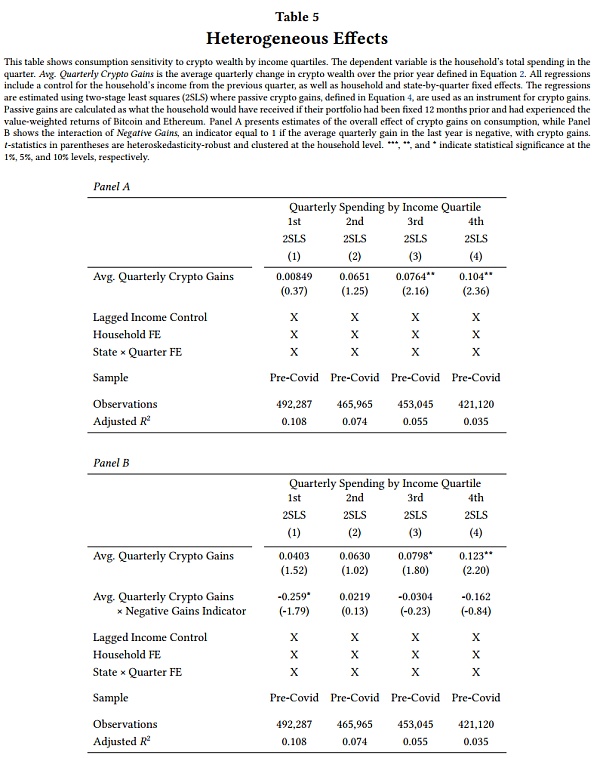
In Panel B of Table 5, this paper examines the asymmetry between cryptocurrency gains and losses in each income quartile. This paper finds no evidence of asymmetry for households in the top three quartiles of income ranks. However, the situation is different for the lowest-income households. For these households, the comprehensive coefficient implies that for every $1 loss in cryptocurrency, low-income households actually increase their consumption by 0.22. Why do low-income households increase consumption after losses? This paper finds that households are more likely to withdraw from cryptocurrency after a loss. Although this is a loss relative to the cryptocurrency portfolio balance 12 months ago, households now have new dollars available in their checking accounts. For low-income households, it seems that converting these illiquid cryptocurrencies into liquid cash makes them more willing to consume.

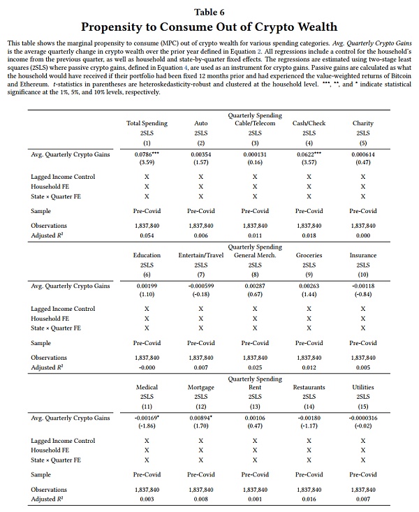
Finally, this paper explores the response of different consumption categories to changes in cryptocurrency wealth in Table 6. The largest impact is on cash/check consumption (see column 4); this consumption accounts for about 80% of total consumption. The remaining consumption effects mainly come from increased mortgage payments. These two results are consistent with the purchase of new homes or other large durables (such as cars), as many expenses associated with home and car purchases are paid by check. In the next section, this paper will further investigate the purchase of new homes.

Table 6 Propensity of Consuming Cryptocurrency Wealth

The results of this section indicate that households change their investment and consumption behaviors after an increase in cryptocurrency wealth. Some households rebalance their portfolios by withdrawing cryptocurrency assets and depositing funds into traditional brokerage firms, while others chase cryptocurrency gains by depositing more funds into cryptocurrency exchanges. The propensity to consume cryptocurrency wealth is 2-3 times higher than that of equity wealth, but lower than that of lottery winnings.

4.1 Study of Cryptocurrency Withdrawal Events

The consumption changes recorded in the previous section occurred after the unrealized changes in cryptocurrency wealth. Consumption decisions following the realization of profits may follow different patterns. According to the data in this article, nearly 50% of cryptocurrency users have withdrawn funds from cryptocurrency exchanges at some point. The decision to realize cryptocurrency profits (i.e., withdrawing funds from cryptocurrency exchanges) is clearly endogenous and may be influenced to some extent by household expenses and balance sheet liquidity. The trend shown in Figure 3 indicates that another factor in cryptocurrency withdrawals is cryptocurrency returns. Overall, withdrawals significantly increase after periods of high Bitcoin returns. Aiello et al. (2023) formally studied this relationship and found that lagged Bitcoin returns positively predict retail cryptocurrency withdrawals. This relationship has led to some changes in household withdrawal decisions.

To evaluate how households change their consumption decisions after withdrawing large amounts of funds from cryptocurrency exchanges, this article models it at the household level using an event study framework. The estimated model in this article is:

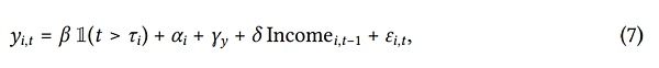
Where the dependent variable yi,t represents the total consumption of different expenditure categories for user i in month t. The main variable of interest is an indicator that equals 1 when month t exceeds the occurrence of a large withdrawal event. In the baseline analysis, this article defines large withdrawals as exceeding $5,000. In the sample used in this article, there are approximately 3,109 such events, with an average withdrawal amount of about $17,000. The regression includes account fixed effects (αi) and year fixed effects (γt), while controlling for lagged monthly income. The analysis is limited to a window of 12 months before and after event ??.

The event study establishes a causal relationship between cryptocurrency withdrawals and changes in consumption. However, this does not establish a causal relationship where withdrawals cause changes in consumption. This is because withdrawal decisions may be made in anticipation of future changes in consumption. If the causal mechanism is expectation-driven withdrawals, it also implies that higher consumption may not be feasible without this additional liquidity. These results suggest that whether it is cryptocurrency withdrawals leading to increased consumption or expected increased consumption leading to the depletion of cryptocurrency wealth, cryptocurrency wealth is used to fund increased consumption.

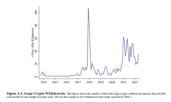
Figure A.4 Large cryptocurrency withdrawals

Appendix Figure A.4 illustrates the number of large cryptocurrency withdrawals over time. There was a sharp increase in large withdrawals during the period of rising cryptocurrency prices in 2017, as well as a noticeable peak in withdrawals after significant returns in early 2021. Despite this intermittent pattern, there have been large withdrawal events almost every month since 2016.

Table 7 Cryptocurrency withdrawals and expenditures

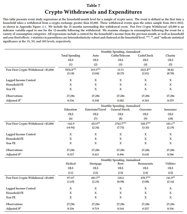
The results in Table 7 report the annualized monthly expenditure differences for various categories after individuals withdraw at least $5,000 from the cryptocurrency market. The coefficient in column 1 indicates that the total expenditure increases by $7,877 relative to the previous year’s expenditure for the household in the year following a large cryptocurrency withdrawal. Unlike expenditure primarily related to virtual cryptocurrency wealth income, expenditure in almost all expenditure categories has significantly increased. This article particularly observes a significant increase in cash/check expenditure and general merchandise expenditure. Discretionary expenditures in entertainment, travel, and dining have also increased significantly. Finally, cryptocurrency withdrawals have also been used for housing expenses – mortgage payments increased by about $600, insurance increased by about $180, and utilities increased by about $140. In fact, even though they are less associated with housing, the increase in expenditure on checks and general merchandise may also indicate down payments, performance bonds, and new home furnishings.

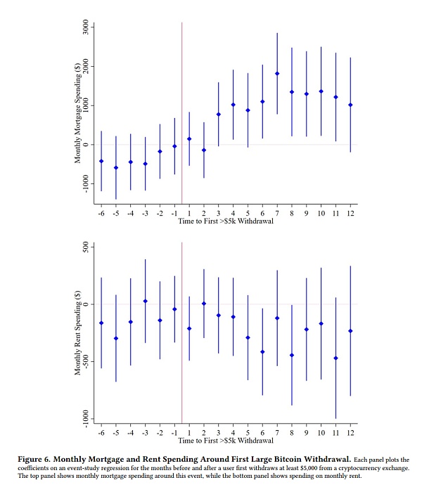
Figure 6 Monthly mortgage and rental expenses before and after the first large Bitcoin withdrawal

Since it seems that many large cryptocurrency withdrawals are used for housing, this article focuses on mortgage expenses in an attempt to understand existing trends that may lead to households cashing out their cryptocurrency wealth. The top panel of Figure 6 shows the mortgage event study, plotting the coefficients relative to the dates associated with the event time after extracting large funds from the cryptocurrency market. Mortgage expenses remained stable in the six months before the large cryptocurrency withdrawal, but increased significantly afterwards. In contrast to mortgage expenses, rental expenses (bottom panel) remained stable within the event window, indicating that the observed increase in spending was not driven by changes in housing prices.

Table 8 Cryptocurrency withdrawals and transition to homeownership

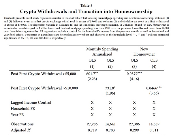
Next, this article examines how the impact of cryptocurrency withdrawals on mortgage expenses varies with different withdrawal amounts. Table 8 reports the mortgage expense results estimated using the model in Equation 7, but with the threshold for large withdrawals increased from $5,000 to $10,000. Columns 1 and 2 show that larger cryptocurrency withdrawal amounts subsequently lead to larger increases in mortgage expenses. For example, users who withdraw at least $10,000 from the cryptocurrency market see an increase in mortgage expenses of $732 in the following year, an estimated effect that is about 20% larger than that for withdrawals of at least $5,000.

The increase in mortgage expenses may be driven by new home purchases, but it could also represent households prepaying existing mortgages. In columns 3 and 4 of Table 8, this article re-estimates the event study using indicators for new home buyers as the outcome variable. This article defines a monthly indicator that equals 1 if a household pays a total mortgage amount exceeding $2,500 in the six months following the cryptocurrency withdrawal and pays less than $100 in total mortgage amount in the six months before the withdrawal. Using this indicator as a proxy for new home purchases, this article finds that a cryptocurrency withdrawal of at least $10,000 increases the probability of entering homeownership by about 4.7 percentage points, representing an approximately 43% increase relative to the sample mean.

The overall impact of cryptocurrency wealth on local housing prices

In Section 4, this article demonstrates that an increase in cryptocurrency wealth leads to increased housing expenditures for households. Individual-level housing decisions may exert price pressures on the local housing market, particularly as Figure 4 shows that household cryptocurrency wealth has geographic concentration. In this section, the article explores the extent to which changes in overall cryptocurrency wealth affect the local housing market. The article first defines monthly county-level cryptocurrency wealth as

where CryptoWealth?,t is the cryptocurrency wealth of household ? at the end of month t as defined in Equation 1, and county-level cryptocurrency wealth CryptoWealthc,t equals the sum of all household cryptocurrency wealth residing in county c at the end of month t. Unlike the household-level analysis in this article, where the sample of households is small, county-level cryptocurrency wealth is aggregated over the entire user transaction database, but only for users that are flagged as high-quality by the data provider. This process results in a sample of approximately 10% of users, or approximately 6 million households.

Then, this article defines the annual county-level cryptocurrency income per person as:

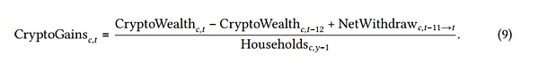
NetWithdrawc,?-11→t is the total sum of cryptocurrency withdrawals minus deposits made by county c in the previous 12 months. Similar to the cryptocurrency income measured at the individual level in this article, CryptoGainsc,t includes both realized and unrealized gains made by county c in the previous 12 months. This indicator is scaled by the number of households in the county’s trading data at the end of the previous year. Assuming that the trading data in this article represents a random sample for each county, this scaling allows for an unbiased estimate of per capita retail cryptocurrency income at the county level, enabling comparisons across different housing market sizes.

This article examines the relationship between county-level cryptocurrency income and housing prices by estimating a regression model of the following form:

ZHVIc,t is the monthly county-level Zillow Home Value Index (ZHVI). County (?c) and year-month (?t) fixed effects control for differences in county wealth levels and national trends in housing prices. This article also includes lagged monthly ZHVI to control for dynamics in the local housing market. Standard errors in this article are clustered at the county level, and the regression is weighted by the ratio of county users to the total county population to mitigate errors caused by sparse sampling.

In order to recover the causal effect of county-level cryptocurrency wealth growth on housing prices, the growth of county-level cryptocurrency wealth in the previous year must be unrelated to future housing prices. There are two reasons why this is unlikely. First, equation 10 may exhibit reverse causality – an increase in housing prices in a certain area may lead households to sell cryptocurrency to purchase homes, thereby reducing the value of the county-level cryptocurrency portfolio. Instantaneous OLS estimates may be biased due to the variation in cryptocurrency prices after these withdrawals. Second, counties that become wealthier are likely to experience increases in housing prices and may also have larger cryptocurrency deposits. This omitted variable may cause the OLS estimates in this article to be upward biased.

To address these issues, this article utilizes the heterogeneity in county-level historical cryptocurrency participation to conduct two natural experiments – the difference-in-differences method and instrumental variable approach – to identify the causal effect of cryptocurrency wealth on local housing prices.

5.1 Difference-in-Differences Method

To study the impact of cryptocurrency portfolio value growth on county-level housing prices, this article first employs the difference-in-differences method to analyze the significant increase in Bitcoin prices at the end of 2017. Throughout the year, the price of Bitcoin rose from $954 to $14,003, an increase of nearly 1,400%, making it the largest 12-month increase in the sample of this article. Several characteristics of the Bitcoin price increase make it an ideal setting to study the impact of cryptocurrency wealth growth on the local housing market.

Firstly, during this period, the huge returns of Bitcoin have significantly increased the crypto wealth of early investors. Secondly, during this period, crypto investments were mainly dominated by Bitcoin – as of December 2016, Bitcoin accounted for 87% of all cryptocurrencies based on market value. This makes the speculative measurement of crypto wealth in this article more accurate during this period compared to later periods when other cryptocurrencies became more developed. Finally, the rise in Bitcoin prices has also led to large-scale withdrawals from crypto exchanges. Evidence in Section 4.1 of this article suggests that large-scale withdrawals are often used to purchase real estate. Inspired by this idea, this article compares the housing prices in counties with high levels of crypto wealth before the price increase with the housing prices in counties with low levels of crypto wealth in the months following the price increase. Formally, this article estimates

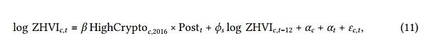
Here, HighCryptoc,2016 refers to the counties that ranked in the top one-third of per capita crypto wealth in December 2016. This article excludes the middle one-third of per capita crypto wealth from the sample.

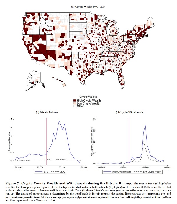
Figure 7 Crypto Wealth and Withdrawals in Counties During Bitcoin Price Increase

Panel a of Figure 7 shows the geographical distribution of counties with high and low crypto wealth in the sample. Postt is an indicator variable that takes the value of 1 when it is in the months following the price increase of Bitcoin. Panel b of Figure 7 shows that the growth rate of Bitcoin prices started to increase significantly in May 2017; therefore, this article defines month 0 as the late period. This article includes an 18-month window around this event and defines Postt as a county-month indicator variable starting from May 2017, with a value of 1. Panel c of Figure 7 confirms the impact on high crypto wealth counties under the shock of Bitcoin; during the late period, the withdrawal volume in these counties increased significantly, while the withdrawal volume in low crypto wealth counties changed less.

In order to confirm the causal impact of crypto wealth changes on housing prices through this method, this article must assume that if Bitcoin prices did not soar, the growth trends of housing prices in high and low crypto wealth counties would be similar. To test this assumption of parallel trends, in Figure 8, this article plots the results of the coefficients estimated by interacting the version of equation 11 with the crypto price shock indicator variables for each month around the 18-month window. This article omits the event month t = -1. The estimated coefficients of the interaction are small and negative in the early period, and not significantly different from zero. In contrast, after the withdrawals began, these coefficients are positive and significant.

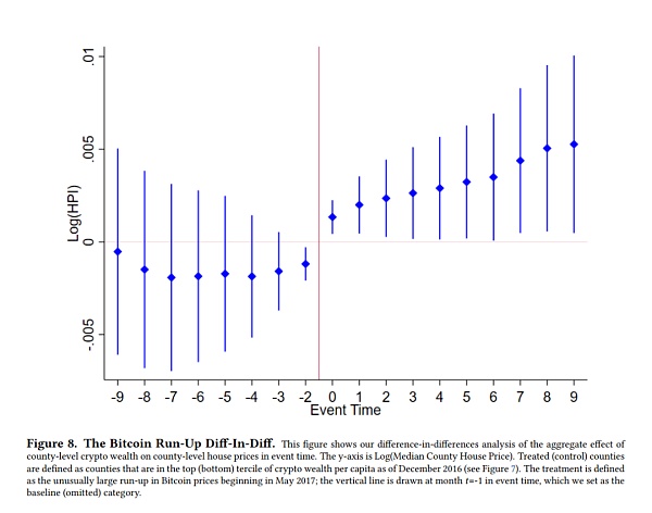
Figure 8 Parallel Trends Test

An important residual question is whether there are other events that occurred simultaneously with the rise of Bitcoin and had differential impacts on housing prices in high and low crypto wealth counties. Given the volatility of Bitcoin, the timing and magnitude of its rise can be considered random. However, the concentration of crypto wealth in counties is not random. Since this article focuses on historical county-level crypto wealth, there is no issue of reverse causality (i.e., the increase in housing prices in 2018 did not cause changes in the value of crypto portfolios in 2016). However, the selection of historical crypto wealth may be correlated with other time-varying county-level characteristics, which could mislead the interpretation of the experiment in this article.

Figure 7 panel a shows the geographical distribution of high and low cryptocurrency wealth counties, which is a potential issue. Although there is significant variation in domestic cryptocurrency wealth, most coastal areas are composed of high cryptocurrency wealth counties. These regions are wealthier and have higher levels of stock market participation. If the correlation between stock returns and cryptocurrency returns is high enough, the differential difference estimates in this paper may reflect the impact of stock wealth rather than cryptocurrency wealth. To mitigate concerns that the differential comparison experiment in this paper may be influenced by stock returns, this paper takes three steps.

First, this paper compares Bitcoin returns with NASDAQ returns during several months of cryptocurrency wealth shocks (see Appendix Figure A.2). Although Bitcoin returns during this period are 20-50 times higher than NASDAQ returns, NASDAQ returns are quite high for stocks, ranging from 20% to 30%. Importantly, NASDAQ returns are relatively stable during cryptocurrency wealth shocks, and even decline.

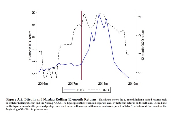
Figure A.2 Bitcoin and NASDAQ 12-month rolling returns

Second, although high cryptocurrency wealth counties experienced a large amount of cryptocurrency withdrawals after Bitcoin price increases, Appendix Figure A.3 shows no discontinuous changes in withdrawals from brokerage accounts around this event, indicating that high cryptocurrency wealth counties did not realize significant stock returns. Finally, the difference-in-differences results of this paper have also undergone robustness tests controlling for county-level stock exposure and lagged indicators.

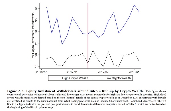
Figure A.3 Equity investment exits around Bitcoin triggered by cryptocurrency wealth

In Table 9, this paper uses the indicator of high cryptocurrency wealth counties to estimate the traditional DID coefficient (columns 1 and 3), as well as the continuous version of interacting lagged indicators with log of per capita cryptocurrency wealth in 2016 (columns 2 and 4). Under both specifications, high cryptocurrency wealth counties experience higher house prices in the months following Bitcoin price increases compared to low cryptocurrency wealth counties.

Table 9 Bitcoin Price Rise DID: County-Month House Prices

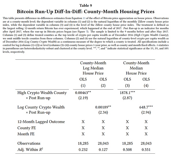
The estimated effects of cryptocurrency wealth on county-level house prices in column 1 suggest that house prices in high cryptocurrency wealth counties grow approximately 46 basis points faster than in low cryptocurrency wealth counties, which is roughly 12% of the standard deviation of house price growth in 2018. In dollar terms, the estimated results in column 3 suggest that in the nine months following Bitcoin price shocks, house prices in high cryptocurrency wealth counties are approximately $1878 higher. This is roughly a 1% increase relative to the mean value of county-level house prices. The continuous specification implies similar but smaller economic magnitudes. Based on the elasticity estimated from changes in county-level cryptocurrency wealth from the 25th to the 75th percentile, house prices will increase by approximately 19 basis points.

5.2 Instrumental Variable Strategy

This paper extends the DID experiment to the entire time series by using the two-stage least squares (2SLS) method. This paper constructs an instrumental variable, CryptoGainsc. Specifically, this paper uses the passive income at the county level to construct the instrumental variable for county-level cryptocurrency assets. The calculation method is to multiply the net income of Bitcoin-Ethereum for the past year by the weighted cryptocurrency wealth of the county 12 months ago:

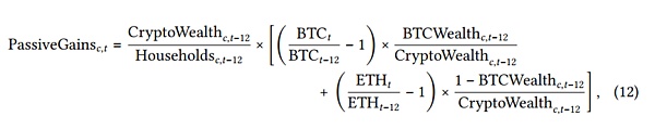
Here, HighCryptoc represents the price of Bitcoin at the end of 2016. This instrument can be interpreted as the change in per capita cryptocurrency assets in the county caused solely by the initial allocation performance of the county towards cryptocurrencies in the past 12 months. This instrument deals with the reverse causality by using the net US dollars earned from the county’s cryptocurrency portfolio without depositing or withdrawing any additional funds within a year.

In order to successfully mitigate concerns about the broader changes in county wealth simultaneously driving cryptocurrency investment and housing prices, the passive income from cryptocurrency wealth (due to the returns of Bitcoin and Ethereum in the past year as well as the heterogeneity in lagged cryptocurrency wealth) must be unrelated to any other changes in non-cryptocurrency wealth that may affect housing prices, controlling for year, month, and county fixed effects. This exclusion restriction may be satisfied for many sources of wealth. For example, due to the quasi-random timing of Bitcoin returns and changes in the county’s occupation or industry mix, these returns are unlikely to be correlated with wealth growth. The remaining reasonable concern is that Bitcoin or Ethereum returns are correlated with equity returns, and the county-level heterogeneity in cryptocurrency wealth is also correlated with heterogeneity in equity wealth. To alleviate this concern, this paper constructs an alternative instrument that represents the passive excess returns of Bitcoin and Ethereum portfolio relative to the stock market returns (NASDAQ, QQQ) during the same period:

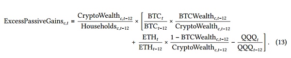
According to this definition, the instrument in this paper represents the passive excess returns of investors’ Bitcoin and Ethereum portfolio relative to the returns of the Nasdaq (QQQ). This modified result produces 31 estimates of the additional effect of county-level cryptocurrency wealth relative to the allocation to similar large technology companies. Using ExcessLianGuaissiveGainsc,t as the instrument yields similar results, indicating that equity returns are not driving the results of this paper. Using these exogenous cryptocurrency returns as instruments, this paper estimates the first-stage regression:

Unsurprisingly, the initial returns of cryptocurrency holdings strongly predict county-level cryptocurrency returns – the first-stage F-statistic ranges from 3000 to 6000 in the main specification of this paper. Then, this paper estimates the following second-stage regression using the predicted cryptocurrency returns from equation 14:

This paper measures the change in the housing price index for the three months after the current month, represented as ZHVIc,t.

Table 10 reports the 2SLS results estimated in equation 15. This study finds that the growth of county-level crypto wealth leads to an increase in county-level housing prices in the next 3 months, and even more in the next 6 months. These estimates are highly significant statistically and robust with fixed effects, whether using LianGuaissiveGains or ExcessLianGuaissiveGains instruments.

Table 10: Impact of cryptocurrency returns on housing prices

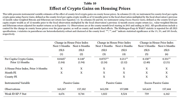
Table 10 results show that an increase of $1 in per capita crypto wealth income in each county would lead to an increase in housing prices of approximately $0.076 in the next 3 months, or about $0.21 in the next 6 months. These estimates imply that an increase of one standard deviation in per capita crypto income would result in an increase of $674 in county housing prices in the next six months. This is approximately 36 basis points higher than the sample average and is roughly consistent with the estimates obtained from DID analysis.

In summary, the evidence from this section and section 5.1 suggests that crypto wealth has spillover effects on the real economy. Counties exposed to crypto assets experience faster housing price growth after large crypto returns.

Conclusion

Increasing numbers of households in the United States are incorporating cryptocurrency as part of their investment strategy, partly due to its extreme volatility leading to rapid wealth accumulation for some investors. This study is the first to document the response of consumer spending to this emerging crypto wealth and identify its spillover effects on local housing prices. Using financial transaction-level data from millions of U.S. households, this study shows that household crypto investors appear to view cryptocurrency as part of their investment portfolio, with some households chasing crypto returns and others rebalancing some crypto returns into traditional brokerage investments. Households also use crypto wealth to increase their discretionary consumption. The tendency to consume crypto wealth is much higher than equity wealth but lower than lottery winnings.

Households also withdraw crypto returns to purchase housing, including becoming new buyers and upgrading existing homes. This increase in housing expenditure puts upward pressure on local housing prices, particularly in areas heavily exposed to crypto assets. Overall, the growth of county-level crypto wealth leads to an increase in county-level housing prices.

According to cryptocurrency advocates, cryptocurrency returns are largely unrelated to other asset classes. Furthermore, the recent collapse of the cryptocurrency market appears to have limited contagion effects on the broader financial markets. While the spillover effects of cryptocurrency on other financial assets may be limited, the results of this study indicate that crypto investments do indeed impact real assets. Therefore, the distribution of crypto wealth has significant implications for the real economy.

Below are screenshots of the article:

We will continue to update Blocking; if you have any questions or suggestions, please contact us!