Understanding the Pros and Cons of FPGA and GPU Acceleration for Zero-Knowledge Proof Calculation

FPGA vs GPU for Zero-Knowledge Proof Calculation: Pros and Cons

Zero-knowledge proof (ZKP) technology is becoming more and more widely used, including privacy proof, computation proof, consensus proof, etc. While looking for more and better application scenarios, many people have gradually realized that the performance of ZKP proof is a bottleneck. The Trapdoor Tech team has been deeply researching zero-knowledge proof technology since 2019 and has been exploring efficient acceleration schemes for zero-knowledge proof. GPU or FPGA is a more common acceleration platform on the market. This article starts with the calculation of MSM, analyzes the advantages and disadvantages of FPGA and GPU in accelerating zero-knowledge proof calculation.

Abstract

ZKP is a technology with a broad future prospects. More and more applications are beginning to adopt zero-knowledge proof technology. However, there are many ZKP algorithms, and various projects use different ZKP algorithms. At the same time, the computational performance of ZKP proof is relatively poor. This article analyzes the MSM algorithm, elliptic curve point addition algorithm, Montgomery multiplication algorithm, etc., and compares the performance differences of GPU and FPGA in BLS 12_381 curve point addition. Overall, in terms of ZKP proof calculation, in the short term, GPU has obvious advantages, high throughput, high cost-effectiveness, programmability, etc. FPGA has certain advantages in power consumption. In the long run, FPGA chips suitable for ZKP calculation may appear, and ASIC chips customized for ZKP may also appear.

ZKP algorithm complexity

ZKP is a general term for zero-knowledge proof technology. It is mainly divided into two categories: zk-SNARK and zk-STARK. The commonly used algorithm for zk-SNARK is Groth 16, PLONK, PLOOKUP, Marlin, and Halo/Halo 2. The iteration of zk-SNARK algorithm mainly goes along two directions: 1/ whether a trusted setup is needed 2/ circuit structure performance. The advantage of zk-STARK algorithm is that no trusted setup is needed, but the verification calculation amount is logarithmically linear.

From the perspective of the application of zk-SNARK/zk-STARK algorithm, the zero-knowledge proof algorithms used by different projects are relatively scattered. In the application of zk-SNARK algorithm, because PLONK/Halo 2 algorithm is universal (no trusted setup is required), more and more applications may be used.

• Web3 IP: What’s Next?
• Deep analysis of the intent behind SEC’s lawsuit against Binance: a jurisdictional dispute or a show of power?
• Apple Vision Pro priced at 25,000 yuan released, ushering in the next generation of human-computer interaction?

PLONK proof calculation amount

Take PLONK algorithm as an example to analyze the calculation amount of PLONK proof.

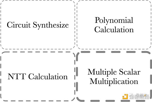
The computational cost of the PLONK proof consists of four parts:

1/ MSM – Multiple Scalar Multiplication. MSM is often used to calculate polynomial commitments.

2/ NTT calculation – transformation of polynomials between point-value and coefficient representation.

3/ Polynomial calculation – polynomial addition, subtraction, multiplication, division, and evaluation, etc.

4/ Circuit Synthesize – circuit synthesis. The computation of this part depends on the size/complexity of the circuit.

Generally, the computational cost of the Circuit Synthesize part is determined by judgment and loop logic, and is more suitable for CPU calculation because of its lower parallelism. Generally, the acceleration of zero-knowledge proofs refers to the acceleration of the first three parts of the calculation, of which the calculation of MSM is relatively the largest, followed by NTT.

What’s MSM

MSM (Multiple Scalar Multiplication) refers to the calculation of the point obtained by adding the results of a given set of points on an elliptic curve with scalars.

For example, given a set of points on an elliptic curve:

Given a fixed set of Elliptic curve points from one specified curve:

[G_ 1, G_ 2, G_ 3, …, G_n]

and random scalars:

and a randomly sampled finite field elements from specified scalar field:

[s_ 1, s_ 2, s_ 3, …, s_n]

MSM is the calculation to get the Elliptic curve point Q:

Q = \sum_{i= 1 }^{n}s_i*G_i

The industry generally uses the Pippenger algorithm to optimize the MSM calculation. Take a closer look at the flowchart of the Pippenger algorithm:

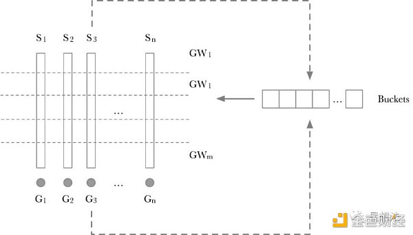
The calculation process of the Pippenger algorithm is divided into two steps:

1/ Scalar splitting into windows. If the scalar is 256 bits and the window is 8 bits, all scalars are divided into 256/8 = 32 windows. For each layer of windows, a “Buckets” is used to temporarily store intermediate results. GW_x is the accumulated result point for a layer. Calculating GW_x is relatively simple. Traverse each Scalar in a layer in turn, use the value of Scalar as the Index for the corresponding G_x to be added to the corresponding Buckets bit. The principle is actually quite simple. If the coefficients of two points added are the same, the two points are added first, and then Scalar is added again, instead of adding Scalar twice for two points before accumulation.

2/ The points calculated for each window are accumulated through double-addition to obtain the final result.

There are many variations of the Pippenger algorithm, but the underlying calculation of the MSM algorithm is point addition on an elliptic curve. Different optimization algorithms correspond to different numbers of point additions.

Elliptic Curve Point Addition (Point Add)

You can see various algorithms for point addition on elliptic curves with “short Weierstrass” form at:

http://www.hyperelliptic.org/EFD/g 1 p/auto-shortw-jacobian-0.html#addition-madd-2007-bl

Assuming the projective coordinates of two points are (x 1, y 1, z 1) and (x 2, y 2, z 2), the result of point addition (x 3, y 3, z 3) can be calculated by the following formula:

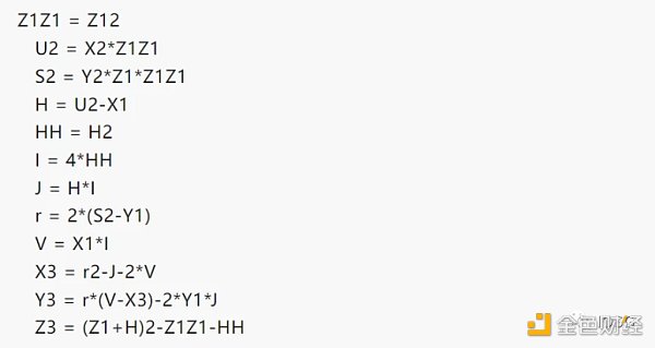
The reason for giving a detailed calculation process is to show that most of the calculation process is integer calculation. The bit width of integers depends on the parameters of the elliptic curve. Here are some common bit widths of elliptic curves:

• BN 256 – 256 bits

• BLS 12 _ 381 – 381 bits

• BLS 12 _ 377 – 377 bits

• It is noteworthy that these integer calculations are modulo operations. Modulo addition/subtraction are relatively simple, but the focus is on the principles and implementation of modulo multiplication.

Modular Multiplication

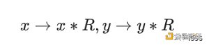
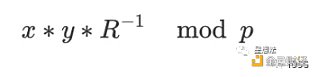
Given two values in the modulo domain: x and y. Modular multiplication refers to x*y mod p. Note that the bit width of these integers is the bit width of the elliptic curve. The classic algorithm for modular multiplication is Montgomery multiplication. Before performing Montgomery multiplication, the multiplicand needs to be converted to Montgomery representation:

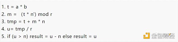
The formula for Montgomery multiplication is as follows:

There are many implementation algorithms for Montgomery multiplication: CIOS (Coarsely Integrated Operand Scanning), FIOS (Finely Integrated Operand Scanning), and FIPS (Finely Integrated Product Scanning), etc. This article does not delve into the details of various algorithm implementations, and interested readers can study them on their own.

To compare the performance differences between FPGA and GPU, the most basic algorithm implementation method was chosen:

Simply put, the modulo multiplication algorithm can be further divided into two types of calculations: large number multiplication and large number addition. Understanding the calculation logic of MSM, the performance (Throughput) of modulo multiplication can be selected to compare the performance of FPGA and GPU.

Observation and Thinking

Under such FPGA design, the Throughput of the entire VU 9 P that can be provided in the BLS 12_381 elliptic curve point addition can be estimated. One point addition (add_mix method) requires about 12 modulo multiplications. The system clock of FPGA is 450 M.

Under the same modulo multiplication/modulo addition algorithm and using the same point addition algorithm, the point addition Troughput of Nvidia 3090 (considering data transmission factors) exceeds 500 M/s. Of course, the calculation involves multiple algorithms, and some algorithms may be suitable for FPGA, and some algorithms may be suitable for GPU. The reason for comparing using the same algorithm is to compare the core computing power of FPGA and GPU.

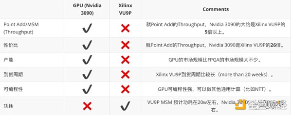
Based on the above results, summarize the comparison of GPU and FPGA in terms of ZKP proof performance:

Summary

More and more applications are beginning to use zero-knowledge proof technology. However, there are many ZKP algorithms, and different projects use different ZKP algorithms. From our practical engineering experience, FPGA is an option, but currently GPU is a cost-effective option. FPGA prefers deterministic calculations, with the advantages of latency and power consumption. GPU has high programmability, a relatively mature high-performance computing framework, short development and iteration cycles, and prefers throughput scenarios.

We will continue to update Blocking; if you have any questions or suggestions, please contact us!