Understanding the Zero Knowledge Proof Algorithm Zk-stark – Arithmetization

Foreword

The first article in this series ( https://www.8btc.com/article/512859 ), with Zk-snark as a comparison, gives a general introduction from the concept and algorithm flow. It is recommended to read the contents of the first article before reading this article. In this article, let us embark on a journey of exploring the mysteries of the Zk-stark algorithm from the shallower to the deeper.

review

In the first article, the Zk-stark algorithm can be roughly divided into two parts: Arithmetization and Low Degree Testing. In this article, we first detail the first phase of the algorithm, Arithmetization.

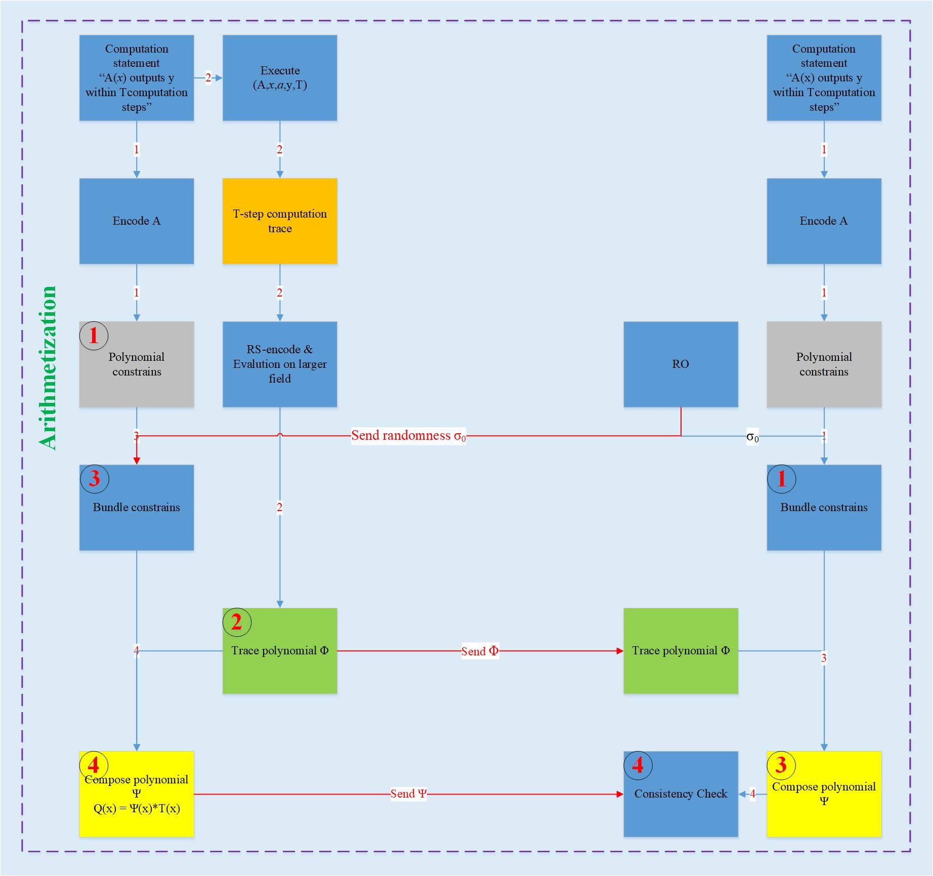
The overall steps of Arithmetization are shown below:

• Galaxy Digital launches two new funds targeting 1% of the wealthy
• Blockchain talent shortage: annual salary of 200,000, unable to recruit blockchain engineers
• Financial Times: The global blockchain market is developing rapidly China may have more voice

So what is Arithmetization? What is the specific process? With these questions, let us carefully taste the content behind the article.

First of all, what is Arithmetization?

Arithmetization is the process of transforming a CI statement into a formal Algebraic language. This step has two purposes: first, presenting the CI statement in a clear and concise manner; second, embedding the CI statement in the algebraic domain for the latter polynomial Conversion is a bedding. The Arithmetization representation consists of two main parts: first, the execution trajectory (the orange part of the figure); second, the polynomial constraint (the gray part of the figure). The execution trajectory is a table, and each row of the table represents a single-step operation; the construction of the polynomial constraint is complementary to the execution trajectory, that is, only when the execution trajectory is correct, the polynomial constraint will satisfy each row of the execution trajectory. Finally, the execution trajectory and polynomial constraints are combined to form a certain polynomial, and then the polynomial is LDT verified. At this point, the problem of verifying the CI statement translates into the problem of verifying the deterministic polynomial LDT.

Arithmetization

Knowing the overall flow of Arithmetization, let's discuss the specific process. For ease of understanding, we use a simple example to run through the entire Arithmetization process.

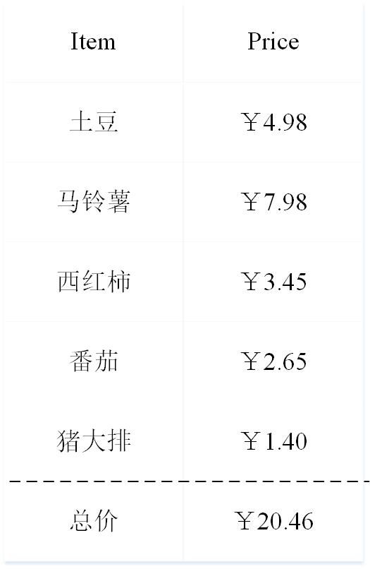
Everyone has been to the supermarket. The contents of the general supermarket receipt are as follows:

Now, Hollywood popular actor Bob claims: "the total sum we should pay at the supermarket was computed correctly". How to verify it? In fact, it is very simple. At this time, another actor Alice can complete the verification by simply adding and summing each receipt. Well, this is just a very simple example. In fact, Alice only needs 5 steps to complete the verification process. Imagine such a scene: After all, Bob is very rich and bought 1,000,000 things in the supermarket. Similarly, he claimed: "the total sum we should pay at the supermarket was computed correctly". At this time, Alice is really angry. How to verify, according to the previous method, it must be about 1000000 steps, trouble? Who loves who to do. Bob also felt bad about Alice, after all, for so many years. I thought, is there any way for Alice to make Alice convinced that I am right in a few steps? So, Bob started the strongest brain mode.

Let's use the simple example above to follow Bob to find the way to the calf.

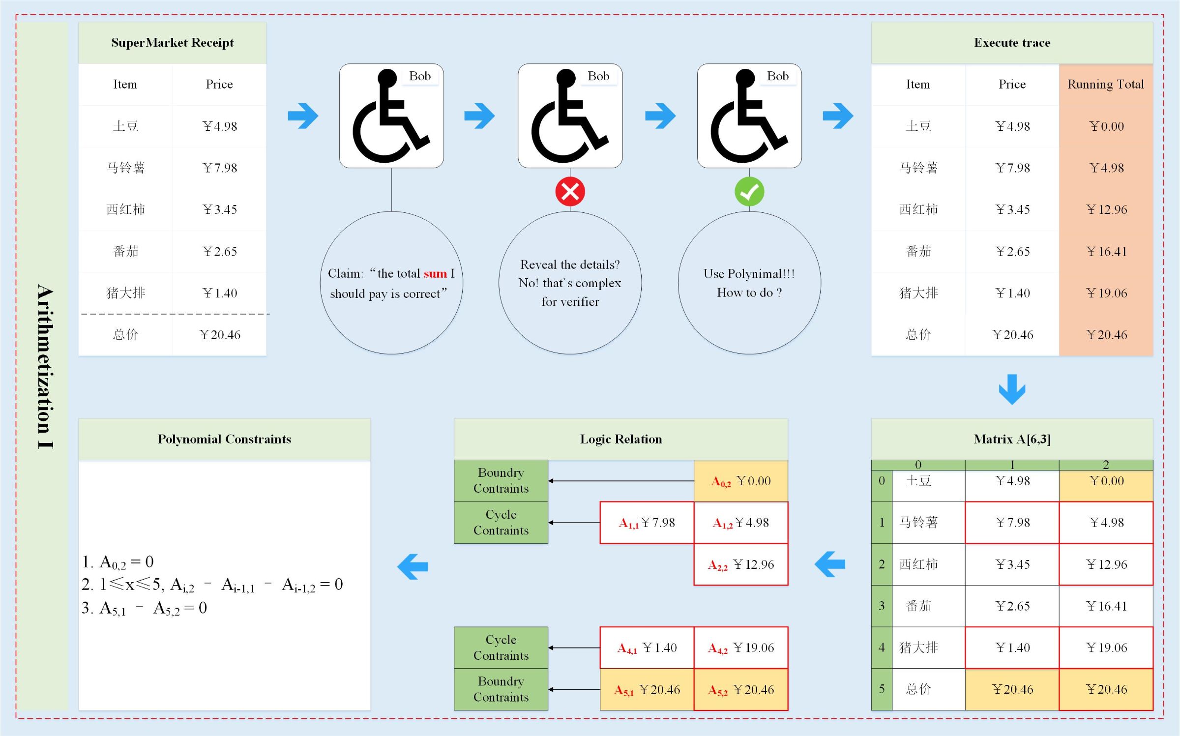
Bob thought, you are not verifying the final sum, right? Then I will list the calculation process of the sum, I promise that the accumulation is correct every time, then my final result must be correct. Bob then added a new column to the receipt to hold the intermediate value in the calculation sum (the orange-brown part of the figure), which is the execution trajectory (the orange part in Figure 1). A new column value needs to be satisfied. The initial value is 0 (the yellow part in Figure 2), the final value is equal to the sum to be paid (the yellow part in Figure 2), and each value in the middle is equal to the previous value plus The unit price of the item in the upper row (the red line in Figure 2), which constitutes the polynomial constraint (the gray part of Figure 1, the lower left part of Figure 2).

As can be seen from Figure 2:

• There are a total of three polynomial constraints, two are boundary constraints (polynomial indexes 1 & 3), and one is a cyclic constraint (polynomial index 2);
• The size of the polynomial has little to do with the answer to the execution trajectory. Even if the length of the table is expanded to 1000000, the final polynomial constraint is still the three, and the only change is the value range of the variable x.

Here, borrowing the words of V God to describe Zk-stark: Zk-Stark is not a deterministic algorithm, it is a large class of cryptography and mathematical structure, with different optimal settings for different applications. It can be understood that for different problems, there are different arithmetic schemes (in this case, one column of values ​​is added, which may not be applicable in other cases), so specific analysis of specific problems is required. But there is a common goal is that no matter what the problem, the resulting execution trajectory is best expressed by a LOOP, so the resulting polynomial constraints are the most concise. The number and form of polynomial constraints directly affect the size of proof and the performance of the Zk-stark algorithm. Therefore, finding an optimal setting is especially important for the Zk-stark algorithm.

Returning to the theme, Bob has now obtained polynomial constraints and execution trajectories, so how do you convert them into a certain polynomial? Please see the picture below: (the blue arrow represents the main flow and the red arrow represents the branch)

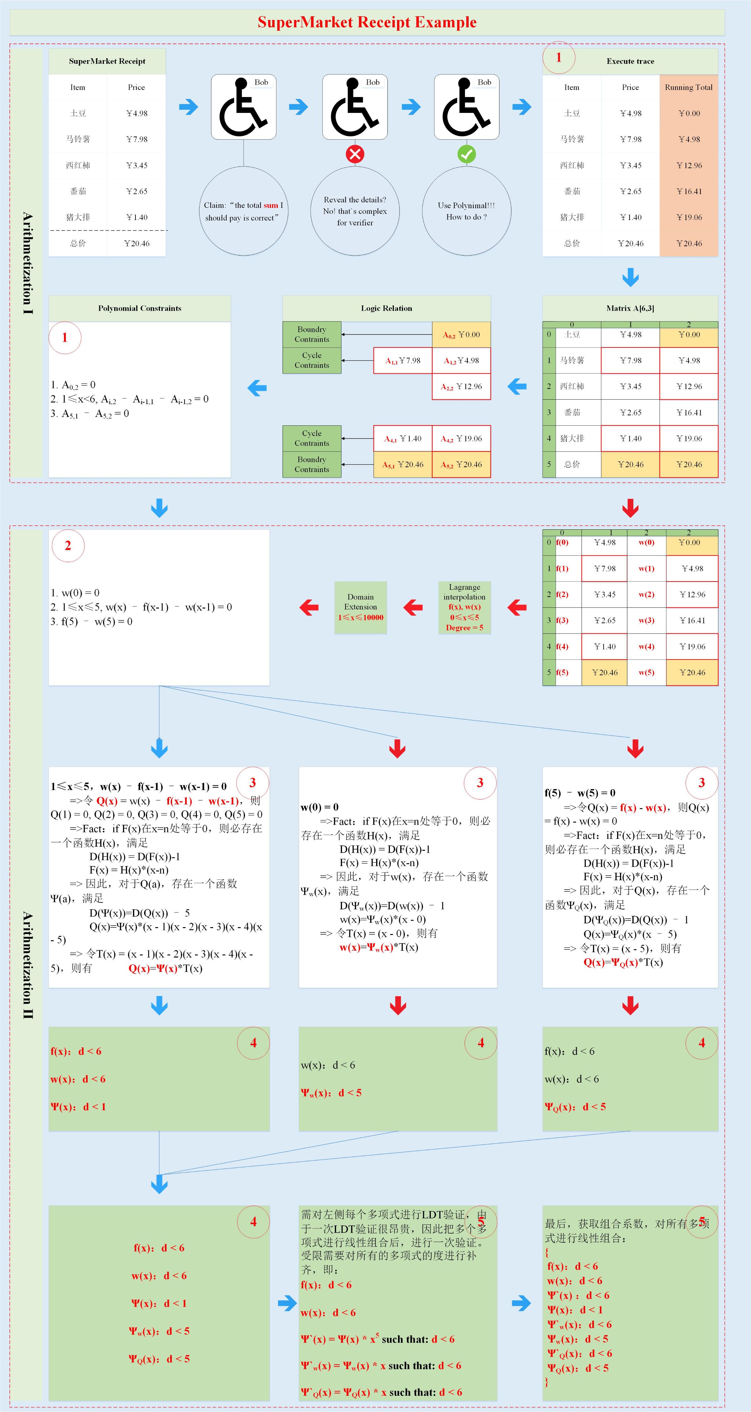
Bob first cuts the focus to the execution trajectory. It can be seen that the execution trajectory has 2 columns, one column is the single item price, and the other column is the price sum. We respectively perform Lagrangian interpolation on the elements of the two columns to get two functions f(x ), w(x), 0≤x≤5. The domain expansion of the two functions is performed separately, and the evaluation at more points is obtained, that is, f(x), w(x), 0≤x≤10000 (from polynomial interpolation to domain expansion, which is actually Reed- Solomen's encoding process, it can be realized, even if there is a difference in the original data, the obtained code words will be very different; the main purpose is to prevent the prover from doing evil, and adding the prover to evil will make the verifier easy to find).

Bob then combines f(x), w(x) and the polynomial constraint equation to obtain a set of exact polynomial constraints (shown by red circle 2 in the figure), taking the circular constraint polynomial as an example:

1 ≤ x ≤ 5 w(x) – f(x -1) – w(x -1) = 0 (1)

Let Q(x) = w(x) – f(x-1) – w(x-1), then Q(1) = 0, Q(2) = 0, Q(3) = 0, Q( 4) = 0, Q(5) = 0.

According to the known fact, the polynomial H(x) of degree d is 0 at x = n, then there exists a polynomial H`(x) of degree d-1, which satisfies d(H`(x)) = d( H(x)) – 1 && H(x) = H`(x) * (x – n)

So for Q(x), the degree is 5, there is a polynomial Ψ(x), the degree is 0, that is, the constant satisfies Q(x) = Ψ(x) * (x – 1)(x – 2)(x – 3) (x – 4)(x – 5), let the target polynomial T(x) = (x – 1)(x – 2)(x – 3)(x – 4)(x – 5), degree 5 , there are:

Q(x) = Ψ(x) * T(x) (2)

The verifier Alice randomly selects a point a from 0 ≤ x ≤ 10000 and sends it to the prover Bob, asking Bob to return the corresponding value. Taking equation (2) as an example, Bob needs to return w(a), w(a-1), f(a-1), Ψ(a), then Alice determines if the equation is true, ie:

w(a) – f(a – 1) – w(a – 1) = Ψ(a) * T(a) (3)

If the equation is true, then Alice has a high probability that the execution trajectory is correct, then the original calculation is true. If the verifier Bob is evil, the 4.98 in the table is changed to 5.98, then Q(1) = w(1) – w(0) – f(0) = 5.98 – 0 – 4.98 = 1, not equal to 0. In this case, observe equation (2), the right side of the equation is Q(x), the degree is 5, and x = 1 is not zero; the right side of the equation Ψ(x) * T(x) , let G(x) = Ψ(x) * T(x), degree is 5, because T(x) is zero at x = 1, so G(x) is also 0 at x=1, so the two sides of the equation are actually Different polynomials with equal degrees have a maximum of 5 intersection points. Therefore, in the range of 0≤x≤10000, only 5 values ​​are equal, and the value of 9995 is unequal. Therefore, a random value is selected from 0≤x≤10000. The probability of verification failure is 99.95%. If the scope of the domain extension is larger, the probability of verification failure will be closer to 1. According to the same logic, the boundary constraint polynomial is processed separately, and the result is shown in the figure (indicated by the red circle 3 in the figure).

Below, we talk about how to add zero knowledge attributes.

For the prover Bob, the execution trajectory is not expected to be seen by the verifier Alice, because it will contain some important information, therefore, the qualified verifier Alice can only randomly select a value from the range of 6 ≤ x ≤ 10000. Verification, of course, this limitation, both parties agree.

There is such a problem. When the verifier Alice receives the value of the certifier Bob's feedback, how to ensure that these values ​​are legal, is indeed calculated by the form of polynomial, and these polynomials are less than a certain degree, instead of the prover Bob only for verification, And the generated random value? For example, how to ensure that w(a), w(a-1), f(a-1), and Ψ(a) are polynomials w(x), f(x), and Ψ(x) at x = a && x = What is the value on a – 1, and the degree of polynomial w(x), f(x), Ψ(x) is less than a fixed value? These questions will be answered in the next article. Before that, let's discuss why the polynomial is less than a fixed value to prove that the original execution trajectory is correct.

From the above example, it can be seen that Q(x) is equal to 0 when x is 1, 2, 3, 4, 5 if and only if the execution trajectory is correct. Then Q(x) can be divisible by the target polynomial T(x), ie: Ψ(x) = Q(x) / T(x) , d(Ψ(x)) = d(Q(x)) – 5 .

As can be seen from Fig. 3, the number of polynomials to be verified is 5 (shown by red circle 4). If LDT is performed for each polynomial, the consumption is very large, so it is possible to linearize these polynomials. Combination (shown by red circle 5), if and only if each polynomial satisfies less than a certain degree, the polynomial after linear combination is also less than a certain degree. This condition is sufficient, and the specific details are shown in the subsequent series. chapter.

Welcome criticism, thank you! !

appendix

1. Official introduction document: https://medium.com/starkware/arithmetization-i-15c046390862

2. Official introduction document: https://medium.com/starkware/arithmetization-ii-403c3b3f4355

We will continue to update Blocking; if you have any questions or suggestions, please contact us!